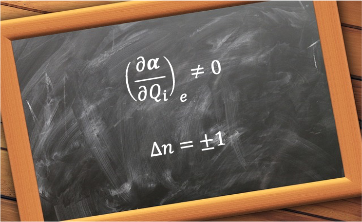
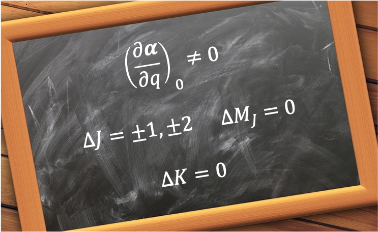
Rotational Raman selection rules describe the allowed changes in a molecule’s rotational angular momentum states during inelastic light scattering.
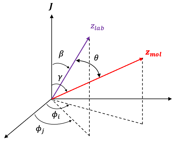
The explicit rotational Raman selection rules for a linear rotor can be derived by considering the molecule with a molecular frame ) interacting with an external electric field
interacting with an external electric field  applied along the laboratory
  -axis (
 ).
).
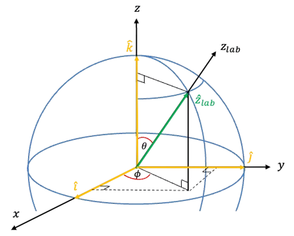
The angle  is the polar angle between the molecular -axis and the laboratory -axis, while
  is the azimuthal angle in the molecular
  -plane, measured from the
  -axis towards the
  -axis (see diagram above).
The first step of the derivation involves expressing the induced dipole moment in terms of the molecular -axis before projecting it onto the direction of the electric field (laboratory -axis).
Simple geometry shows that the direction cosines (the projections of the unit vector  of the laboratory -axis onto the molecular axes) are:

Similarly, the electric field applied along the laboratory -axis has the following components in the molecular frame:

In the molecular frame, the induced dipole moment is a vector  with three components
 ) :
:

where  are the unit vectors along the molecular axes.
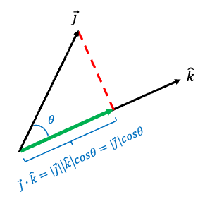
Likewise, the laboratory unit vector can be written in terms of the molecular frame as  . Since the projection of any vector onto a unit vector is given by the dot product between the two vectors (see diagram below), the induced dipole moment
  along the laboratory -axis can be expressed by projecting onto as follows:
\cdot(x\hat{i}+y\hat{j}+z\hat{k})\\&=x\mu_x+y\mu_y+z\mu_z\;\;\;\;\;\;\;\;6\end{align})
Substituting eq4 into eq6 yields:

For a linear molecule, the molecular axes coincide with the principal axes of the polarisability tensor, so that off-diagonal components vanish. Combining  ,
,  and
and  with eq5 and eq7 results in:
)
Replacing  and
and  with
with  , and
, and  with
with  (since the molecular -axis is the parallel axis of rotation, while the molecular – and -axes are the perpendicular axes of rotation), and using
  , gives:
cos^2\theta\;\;\;\;\;\;\;\;7a)
As explained in the previous article, the transition probability associated with scattered radiation is evaluated using  , which in this case, is:
cos^2\theta]\psi sin\theta d\theta d\phi)
where e^{-iM_J^{'}\phi}) and
and e^{iM_J\phi}) are the un-normalised spherical harmonics.
are the un-normalised spherical harmonics.
The integral \phi}) is equal to zero and
is equal to zero and  when
when  and
and  respectively. Thus, we require
  for a probable transition to occur (
 ), resulting in:
)
where
P_{J}^{\vert M_J\vert}(cos\theta)sin\theta d\theta)
P_{J}^{\vert M_J\vert}(cos\theta)sin\theta cos^2\theta d\theta)

 is non-zero when either
  or
or  is non-zero, or when both are non-zero. For the first integral, let
  and
and  , giving:
P_J^{\vert M_J\vert}(x)dx\;\;\;\;\;\;\;\;8)
which is non-zero only if  , or equivalently,

This corresponds to Rayleigh scattering.
The second integral, with and , is:
x^2P_J^{\vert M_J\vert}(x)dx\;\;\;\;\;\;\;\;10)
Substituting the recurrence relation =\frac{J+\vert M_J\vert}{(2J+1)x}P_{J-1}^{\vert M_J\vert}(x)+\frac{J-\vert M_J\vert+1}{(2J+1)x}P_{J+1}^{\vert M_J\vert}(x)) into eq10 yields:
into eq10 yields:
\;\;\;\;\;\;\;\;11)
where
}\int_{-1}^1P_{J^{'}}^{\vert M_J\vert}(x)xP_{J-1}^{\vert M_J\vert}(x)dx)
}\int_{-1}^1P_{J^{'}}^{\vert M_J\vert}(x)xP_{J+1}^{\vert M_J\vert}(x)dx)
Letting  in the same recurrence relation and substituting it into eq11 results in:
)
where
(J^{'}+\vert M_J\vert)}{(2J+1)(2J^{'}+1)}\int_{-1}^1P_{J^{'}-1}^{\vert M_J\vert}(x)P_{J-1}^{\vert M_J\vert}(x)dx)
(J^{'}-\vert M_J\vert+1)}{(2J+1)(2J^{'}+1)}\int_{-1}^1P_{J^{'}+1}^{\vert M_J\vert}(x)P_{J+1}^{\vert M_J\vert}(x)dx)
(J^{'}-\vert M_J\vert+1)}{(2J+1)(2J^{'}+1)}\int_{-1}^1P_{J^{'}+1}^{\vert M_J\vert}(x)P_{J-1}^{\vert M_J\vert}(x)dx)
(J^{'}+\vert M_J\vert)}{(2J+1)(2J^{'}+1)}\int_{-1}^1P_{J^{'}-1}^{\vert M_J\vert}(x)P_{J+1}^{\vert M_J\vert}(x)dx)
 for a linear rotor because
  .
.  and
and  are non-zero only if , which gives the same Rayleigh scattering selection rule as eq9. For
  to be non-zero, we require
  or equivalently,
  . The selection rule corresponding to
  is
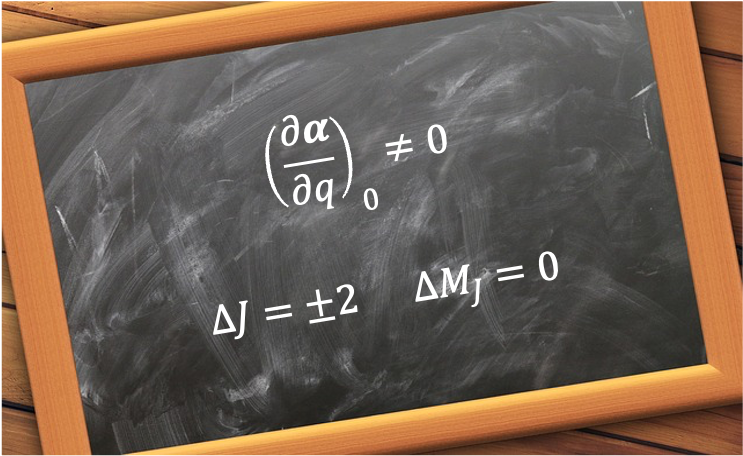
is  . Therefore, the selection rules for rotational Raman transition of a linear rotor are:

The selection rules  can also be explained semiclassically, with the induced dipole moment given by:

where  is the angular frequency of the incident radiation.
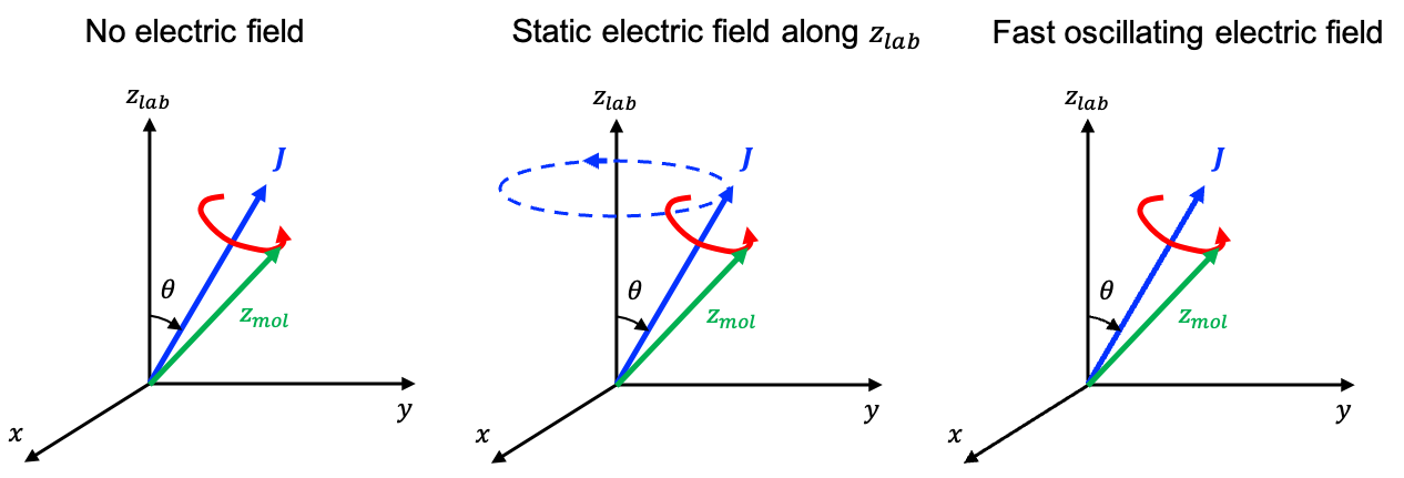
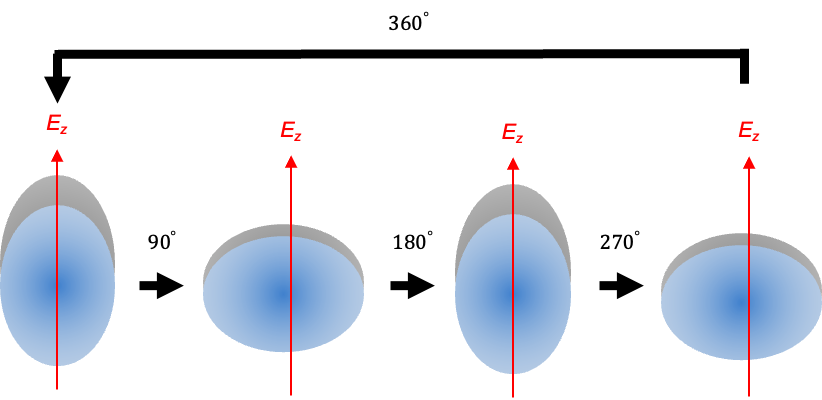
If the linear molecule is rotating an angular frequency  , the value of its polarisability repeats twice per revolution cycle (see diagram above):

where  is the constant baseline (average) polarisability of the molecule.
Substituting eq13 into eq12 gives:
cos(2\omega_rt))
Using the identity +cos(x-y)]) yields:
yields:
t+cos(\omega_i-2\omega_r)t]\;\;\;\;\;\;\;\;14)
Eq14 shows that the induced dipole moment consists of three components: one oscillating at the incident frequency, and two at  . Each time-dependent component of the induced dipole moment corresponds to an oscillating dipole, which radiates electromagnetic energy at the frequency at which it oscillates. It follows that the components oscillating at and give rise to Rayleigh-scattered radiation and Raman-scattered radiation respectively.

Question
Why does each component on the RHS of eq14 correspond to an oscillating, rather than the entire sum corresponding to a single oscillating dipole?
Answer
An oscillating electric dipole is defined by an electric dipole moment that varies sinusoidally in time at a single frequency, for example  . Therefore, eq14 represents a superposition of three independent sinusoidal components, which can be viewed as a Fourier decomposition of the induced dipole moment. Each term oscillates at a distinct frequency and therefore corresponds to an independent oscillating dipole that radiates at that frequency.
Raman selection rules are often discussed for thermally populated rotational levels, where  is typically large (the classical limit). For large , the magnitude of the quantum angular momentum of the molecule is
 }\approx \hbar J) . Substituting this approximation into
. Substituting this approximation into  gives:

 is the angular frequency of a Stokes-scattered photon, which is associated with the resultant quantum rotational transitional frequency of
 =+2\omega_r\approx \frac{2\hbar J}{I}) . This corresponds to the selection rule , because at large ,
. This corresponds to the selection rule , because at large ,
(J+3)-J(J+1)]\\&=\frac{\hbar^2}{I}(2J+3)\approx\frac{2\hbar^2J}{I}\end{align})
Similarly, the angular frequency  (anti-Stokes scattering) leads to the selection rule .