The rotational molecular partition function is a measure of the number of thermally accessible rotational energy states available to a single non-interacting molecule at a specific temperature.
Linear rotors
Consider a heteronuclear diatomic molecule with rotational energies given by eq45: . Substituting this equation into the rotational component of eq257, noting that each energy level is
-fold degenerate, gives:
At low temperatures, is calculated by substituting experimental values of
into eq270. At higher temperatures, such as typical laboratory conditions at room temperature, many rotational energy levels become thermally accessible and populated because
. Since the exponential term varies smoothly with
at room temperature when
, we can simplify eq270 by approximating the sum as an integral:
Substituting and
into eq271 yields
, which evaluates to:
Since has units of Kelvin, eq272 can also be expressed as:
where is known as the characteristic rotational temperature.
Eq273 is valid only when , which is generally true at room temperature. For this reason, it is often referred to as the high-temperature approximation to the rotational partition function.
As discussed in the article on the effect of nuclear statistics on rotational states, nuclear spins dictate which rotational states are populated for symmetrical molecules such as O2 and CO2, resulting in half of all possible rotational states being inaccessible. For such molecules, eq273 becomes:
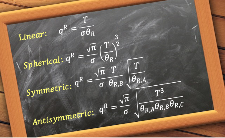
In general, the rotational partition function for all linear rotors can be written as:
where the symmetry number is 1 for non-symmetrical linear molecules like HCl and 2 for for symmetrical linear molecules such as O2 and CO2.

Question
Is unique to rotational partition functions?
Answer
Yes. The symmetry number appears specifically in rotational partition functions. Although we have explained it using quantum mechanics, can also be understood within the framework of classical physics.
At high temperatures, the spacing between rotational energy levels becomes very small compared to , making the discrete quantum levels effectively continuous. The rotational partition function is then approximated classically as an integral over phase space, i.e. over all possible orientations and angular momenta. Here, each energy state corresponds to a particular configuration of positions and momenta. However, for symmetric molecules like CO₂, certain rotational operations (such as a 180° rotation around the molecular axis) produce configurations that are physically indistinguishable. To avoid overcounting these indistinguishable orientations, the symmetry number is introduced as a correction factor in the rotational partition function.
Spherical rotors
The rotational partition function for spherical rotors is derived using the same logic as that for linear rotors. Since the rotational energy levels of a spherical rotor is given by the same expression as that for a linear rotor, the rotational partition function of a spherical rotor, noting that each energy level is -fold degenerate, is given by:
Similar to linear rotors, at low temperatures is calculated by substituting experimental values of
into eq276. At higher temperatures, we apply the high-temperature approximation, with eq276 becoming:
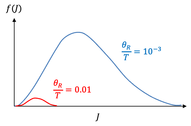
The factor in the function
increases quadratically with
, while
decreases exponentially. It follows that the graph of
versus
forms a skewed bell curve with a maximum. If
, the contribution of
to the integral is negligible at low
and becomes significant only at higher
(see diagram below). Therefore, eq277 can be simplified to:
Question
Prove that for
.
Answer
We shall begin with the identity (see this article for derivation).
So,
Eq278 evaluates to:
Like linear rotors, the symmetry number is added to prevent overcounting of rotational states, giving:
Question
How do we determine the value of for non-linear molecules?
Answer
As mentioned in the previous article, the symmetry number is a correction factor to prevent overcounting indistinguishable classical energy states. A straightforward way to determine is to identify the rotational subgroup to which the non-linear molecule belongs. The order of this group, which is the number of unique proper rotational symmetry operations that map the molecule onto itself, is equal to
. For example, CH4 belongs to the tetrahedral point group
, whose rotational subgroup has an order of 12 (including 11 rotational symmetries and the identity), so
.
Symmetric rotors
The energy equation of a symmetric rotor depends on three quantum numbers: . Therefore, the rotational partition function for symmetric rotors involves three summations:
or equivalently,
Question
Is the total degeneracy of a symmetric rotor or
?
Answer
The rotational partition function sums over all possible rotational states. The total degeneracy of a symmetric rotor is . Here,
comes from the number of
values for a given
, which is accounted for by the most inner sum. The additional factor of 2 comes from the quantum number
, which ranges from
to
. For
, the energy levels associated with
are degenerate. However, these
-dependent energy levels must be summed over explicitly, as not all values of
correspond to the same energy.
The double summation in eq282 involves fixing a value of and summing the allowed values of
. Since
runs from
to
, with
for each
, the minimum allowed value of
for a given
is
. This allows us to change the order of summation in eq282 by fixing a value for
and then summing over the allowed values of
:
Substituting into eq283 and using the high-temperature approximation gives:
Using the earlier argument that if , the contribution of
to the 2nd integral in eq284 is negligible at low
and becomes significant only at higher
, we have
Since , the 2nd integral in eq285 evaluates to
and eq285 becomes:
Using the identity , we have
where we have added the symmetry number (e.g. for NH3), with
and
.
Question
What is the expression for the rotational partition function of an asymmetric rotor?
Answer
An asymmetric rotor has three distinct moments of inertia: . Its rotational energy is characterised by three rotational constants:
,
and
. If two of the moments of inertia are equal, the molecule becomes a symmetric rotor. It follows that the rotational partition function of asymmetric rotor is:
which reduces to eq286 when .