Intermediate Chemistry - Mono Mole

November 16, 2019November 16, 2024

Aufbau principle

The Aufbau principle (building up principle) states that an atom in its ground state has electrons filling its orbitals in the order of increasing energy. It was proposed by Niels Bohr and Wolfgang Pauli in the 1920s and is based on the observation that the lower the energy of a system is, the more stable it is.

Specifically, the principle adopts the $n+l$ rule, which was first suggested by Charles Janet in 1928, in his attempt to construct a version of the periodic table. It was later adopted by Erwin Madelung in 1936, as a rule on how atomic sub-shells are filled.

The empirical rule states that electrons fill sub-shells in the order of increasing value of $n+l$ where $n$ is the principal quantum number and $l$ is the angular quantum number. It further mentions that electrons fill sub-shells in the order of increasing value of $n$ for sub-shells with identical values of $n+l$ . For example,

Subshell	${\color{Red} n}$	${\color{Red} l}$	${\color{Red} n+l}$	Order
1s	1	0	1	1
2s	2	0	2	2
2p	2	1	3	3
3s	3	0	3	4
3p	3	1	4	5
3d	3	2	5	7
4s	4	0	4	6

The order of fill is represented by the diagram above. So, the ground state electron configuration (distribution of electrons) for calcium is 1s² 2s² 2p⁶ 3s² 3p⁶ 4s² or [Ar]4s², where [Ar] is the electron configuration of argon. The Aufbau principle works well for elements with atomic number $Z\leq 20$ but must be applied with a better understanding of orbital energy and electron repulsion for $Z>20$ .

For elements with Z between 1 and 6, calculations show that the energy of the 4s sub-shell is higher than the 3d sub-shell (see diagram above). For Z between 7 and 20, the reverse is true, as a result of the interplay between increasing nuclear charge and increasing electron repulsion. The relative energy of the s and d sub-shells again changes for $Z>20$ , where the 3d sub-shell has a lower energy than the 4s sub-shell. This is because electrons in 3d orbitals do not shield each other well from nuclear forces, leading to the lowering of their energies.

With that in mind, one may conclude that the electron configurations of scandium and titanium are [Ar]3d³and [Ar]3d⁴ respectively. However, they are [Ar]3d¹4s²and [Ar]3d²4s². Numerical solutions of the Schrodinger equation for scandium and titanium not only show that the 3d orbitals have lower energies than the 4s orbitals, but also reveal that the 3d orbitals are smaller in size compared to the 4s orbitals. Electrons occupying 3d orbitals therefore experience greater repulsions than electrons residing in 4s orbitals, with the order of increasing repulsion being:

$V\left ( e_{4s},e_{4s} \right )<V\left ( e_{4s},e_{3d} \right )<V\left ( e_{3d},e_{3d} \right )$

where V is the potential energy due to repulsion.

To determine the stability of an atom in the ground state, we need to consider the net effect of the relative energies of 4s/3d orbitals and the repulsion of electrons. In fact, calculations for the overall energies of scandium are as follows:

$E[Ar]3d^14s^2<E[Ar]3d^24s^1<E[Ar]3d^3$

Consequently, when a transition metal undergoes ionisation, the electron is removed from the 4s orbital rather than the 3d sub-shell. Despite 3d being lower in energy than 4s for the first row of transition metals, the $n+l$ rule applies. However, the rule breaks down for chromium and copper, where the ground state electronic configuration of chromium is [Ar]3d⁵4s¹instead of [Ar]3d⁴4s² and that of copper is [Ar]3d¹⁰4s¹ instead of [Ar]3d⁹4s². This is attributed to Hund’s rule.

Next article: Hund’s rule

Previous article: Pauli exclusion principle

Content page of intermediate quantum chemistry

Content page of intermediate chemistry

Main content page

November 16, 2019September 25, 2024

Hund’s rule

Hund’s rule states that electrons occupy orbitals of a sub-shell singly and in parallel before pairing up (see diagram below for the n = 2 shell of carbon). This is sometimes called the ‘bus seat’ rule, where bus passengers who travel alone tend to occupy empty double-seats before partly occupied seats.

By spacing themselves apart in different orbitals, electrons attain a relatively stable configuration. This is because electrons offer one another less shielding from the nuclear charge if they are further apart. The decreased shielding leads to the electrons being stabilised closer to the nucleus, resulting in a lower energy system (see digram below).

But why do the electrons that occupy the p-orbitals singly in the above example have parallel spins? A crude explanation is to visualise an electron with a north pole and a south pole (a dipole) due to the magnetic field that it generates with its spin. To stay far apart from each other to reduce repulsion, the dipoles of the two electrons in the p sub-shell must be aligned in a parallel fashion. If the dipoles are anti-parallel, the electrons will be closer to each other, resulting in a higher and less stable energy state. The proper explanation for Hund’s rule, however, lies in the symmetry of the wave function of the system.

Question

Why can’t the n = 2 electron configuration of carbon be 2s¹2p_x¹2p_y¹2p_z¹?

Answer

The stability of the ground state of carbon is a result of the interplay between Hund’s rule and the Aufbau principle. Since the 2s orbital is of a lower energy than each of the 2p orbitals, the electron configuration of the n = 2 shell of 2s²2p_x¹2p_y¹2p_z⁰ offers greater stability to the system than the configuration of 2s¹2p_x¹2p_y¹2p_z¹.

To understand why the ground state electron configuration of chromium is [Ar]3d⁵4s¹instead of [Ar]3d⁴4s²and that of copper is [Ar]3d¹⁰4s¹instead of [Ar]3d⁹4s², we need to consider the following:-

1. The 3d sub-shell has a lower energy than the 4s sub-shell for Z > 20 (see previous article).
2. Electrons occupying 3d orbitals experience greater repulsions than electrons residing in 4s orbitals (see previous article).
3. Hund’s rule states that electrons prefer to stay apart from one another by occupying orbitals singly before pairing up.

The electronic configuration of a 1^st row transition metal is dependent on the interplay of the above three factors. For chromium, the energy level of the 3d sub-shell is very close to that of the 4s sub-shell and hence the 3^rd factor outweighs the 2^nd one. For copper, the energy level of the 3d sub-shell is much lower than that of the 4s sub-shell such that the 1^st factor outweighs the other two factors.

Next article: Heisenberg’s uncertainty principle

Previous article: Aufbau principle

Content page of intermediate quantum chemistry

Content page of intermediate chemistry

Main content page

November 16, 2019September 25, 2024

Heisenberg’s uncertainty principle

Heisenberg’s uncertainty principle states that the position and momentum of a particle cannot be determined simultaneously with unlimited precision. It was developed by Werner Heisenberg, a German physicist, in 1927 and is expressed mathematically as:

$\Delta p_x\Delta x\geq \frac{\hbar}{2}$

where $\Delta p_x$ is the uncertainty in the x-component of a particle’s momentum, $\Delta x$ is the uncertainty in the particle’s position along the x-axis, and $\hbar=\frac{h}{2\pi}$ .

In other words, the product of the uncertainty in measuring a particle’s momentum and the uncertainty in the simultaneous measuring of the particle’s position is never less than $\hbar/2$ (see here for proof). It is important to note that the uncertainties in the measurements are not due to the limitation of measuring devices but an inherent property of nature.

To explain the uncertainty principle, we turn to de Broglie’s hypothesis, which states that all matter behaves like waves. For an electron, its wave property is described by a wave function, e.g. $\psi=Ae^{ikx}$ , which has a well-defined wavelength $\lambda=\frac{2\pi}{k}$ (since $Ae^{ik\left ( x+\frac{2\pi}{k} \right )}=Ae^{ikx}$ ) and hence a precisely determined momentum $p=\frac{h}{\lambda}=k\hbar$ . Furthermore, the position of the electron, according to the Born interpretation, is given by the probability density $\left | \psi \right |^2$ where

$\left | \psi \right |^2=\psi^*\psi=Ae^{-ikx}Ae^{ikx}=A^2$

The equation above shows that the probability density of the electron is uniform, i.e. the electron has equal probability to be found anywhere along the x-axis. If an electron’s momentum is precisely specified, its location cannot simultaneously be determined.

For the reverse argument, where the position is precisely defined, let’s start with an electron with a wave function, where the wavelength is precisely defined, e.g. $cos\pi x$ (represented by the red curve in diagram I below).

If we linearly add another wave function with a different wavelength $cos2\pi x$ to $cos\pi x$ and divide the sum by two* to maintain the same amplitude as $cos\pi x$ , we have a new wave function $y=\frac{1}{2}cos\pi x+\frac{1}{2}cos2\pi x$ or $\sum_{n=1}^{N}\frac{cosn\pi x}{N}$ where N = 2. This is equivalent to the interference pattern of two superimposed wave functions. If we continue to superimpose the first wave function with more wave functions, each of different wavelength, we end up with the blue curve, the green curve and the black curve, for N =5, N = 20 and N = 100 respectively. It is evident from diagram I that as more wave functions of different wavelengths are linearly added to the first wave function, the spread of the resultant wave function becomes narrower.

* this is done for convenience, so that the resultant curve can fit within our view.

For the N = 5 wave function, the probability of locating the electron within a certain percentage P is $\int \left | \psi \right |^2dx$ , which is the area under the blue curve from x₅ to x+Δx₅ (diagram II). Notice that all curves in diagram II are above the x-axis since they represent the square of the respective wave functions. For the N = 20 wave function, let’s assume that the probability of locating the electron within the same percentage is approximately the area under the green curve from x₂₀ to Δx₂₀ in diagram III (note that the amplitude of the N = 20 function in the diagram is normalised for convenience; rightfully, it is very much higher than the amplitude of the N =5 function, and hence the areas under both peaks are comparable). Clearly, the interval x₂₀ to x+Δx₂₀ is shorter than the interval x₅ to x+Δx₅. Hence, we can locate the electron, with a certain probability P, within a smaller interval as N increases, i.e. the uncertainty in locating the electron becomes smaller as N increases. However, the resultant wave functions of N =5 and N = 20 now consist of 5 and 20 distinct wavelengths respectively. Since each wavelength represent a specific value of momentum, a wave function with a wider spread of wavelengths leads to a greater uncertainty of momentum. In the limit of N → ∞ , we have a precisely localised electron but a completely unpredictable momentum.

Question

The speed of an electron in a one-dimensional space is measured, within 3% accuracy, as 2.20 x 10⁶ m/s. What is the length of the space?

Answer

The minimum uncertainty in the position of the electron is:

$\Delta x\geq \frac{\hbar}{2m\Delta v_x}=\frac{1.055\times10^{-34}}{2\times9.11\times10^{-31}\times0.03\times2.20\times10^6}=8.8\times10^{-10}\, m$

If we assume that there is absolute certainty that the electron is not outside the region of space, the uncertainty in position of the electron must be attributed to the length of space.

Next article: Nuclear spin

Previous article: Hund’s rule

Content page of intermediate quantum chemistry

Content page of intermediate chemistry

Main content page

November 13, 2019December 9, 2024

Photoelectric effect

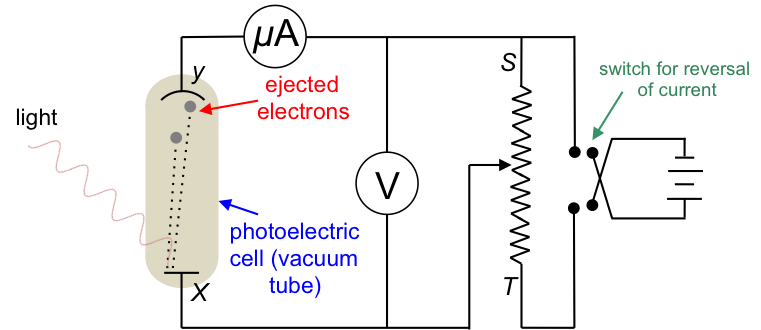
The photoelectric effect is the ejection of electrons from the surface of a material when light strikes it. This occurs due to the transfer of energy from light to the electrons, providing them with sufficient kinetic energy to be ejected from the material. Heinrich Hertz was the first scientist to discover the photoelectric effect in 1887. Since then, other scientists conducted various experiments to study the effect using apparatus similar to the one in the diagram below:

The experiment

The apparatus consists of a photoelectric cell connected to a potentiometer and a battery with a commutator (switch for reversal of current). At the start of the experiment, the potential difference across X and Y is set to zero, i.e. the battery is disconnected from the circuit and the wiper is slid to S. Light of a particular frequency and intensity striking X ejects electrons with different kinetic energies into the vacuum between X and Y, and leaves behind positive charges (holes) at X. The ejected electrons with the proper trajectory reach Y and return along the wire to X, thereby completing the circuit and generating a very small current in the order of a few micro amperes.

Question

Why doesn’t the positively charged holes attract the ejected electrons back to X? Why do the ejected electrons have different kinetic energies?

Answer

Energy has been transferred from the incident radiation to the electrons to overcome the electrostatic forces of attraction. Any electron that leaves X will reach Y if they are ejected at the appropriate angle and not repelled by other electrons in the vacuum tube.

The ejected electrons have different kinetic energies because they reside at different depths of the material’s surface at X prior to ejection. The deeper they are, the lower their kinetic energies upon ejection due to electrostatic (nuclear forces of attraction) and mechanical factors (collisions).

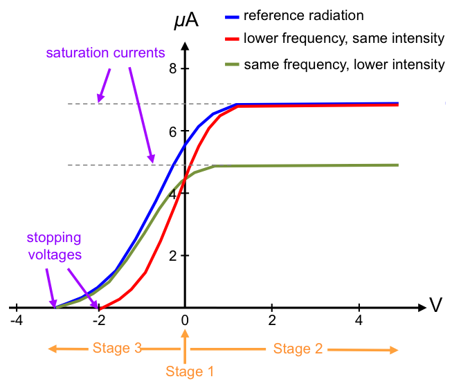
The next stage of the experiment involves connecting the battery to the circuit with its positive terminal to Y and negative terminal to X. The wiper is gradually slid towards T and the current in the circuit increases and reaches a saturation value.

In the last stage of the experiment, the terminals of the battery are connected to the circuit in reverse and the wiper is returned closer to S. X is now positively charged and fewer electrons reach Y, causing the current in the circuit to decrease. As the wiper is again slid towards T, the potential difference across XY increases (the voltmeter reading becomes more negative) and the current decreases further until it drops to zero. The voltage required to completely stop the current from flowing in the circuit is called the stopping voltage. The experiment is then repeated by separately varying the frequency of the incident radiation and the intensity of the radiation.

The RESULTS

When incident radiation above a certain threshold frequency impinges the material (electrode) at X,

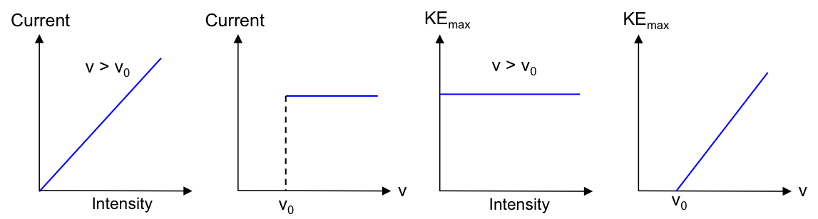
1. the current produced is proportional to the intensity (brightness) of the incident radiation but independent of its frequency.
2. the absolute value of the stopping voltage is proportional to the frequency of the incident radiation but independent of its intensity.
3. the effect is instantaneous, i.e. no time delay between the incidence of light and emission of electrons.

Scientists at that time failed to explain all the results using the wave theory of light, which predicted the following:

The current produced is proportional to the frequency of the incident radiation. This is because wave theory suggests that the oscillating electric field of the incident light causes electrons to oscillate and eventually break free from the material. The higher the frequency of the incident light, the higher the probability of electrons breaking free from the material.
The absolute value of the stopping voltage should be proportional to light intensity, as wave theory defines light intensity as energy/(area x time). Therefore, a higher energy light source should require a stopping potential of a larger magnitude.
There should be a time difference between the ejection of electrons at low light intensity versus high light intensity, because incident light energy is shared throughout the cathode and is cumulative according to classical wave theory (i.e. the amplitude of the oscillation of electrons will increase over time as light waves continue to hit the cathode until the electrons have the required energy to be ejected).

EXPLANATION OF RESULTS

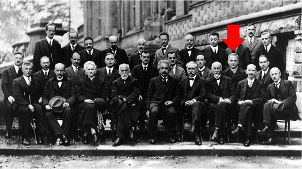
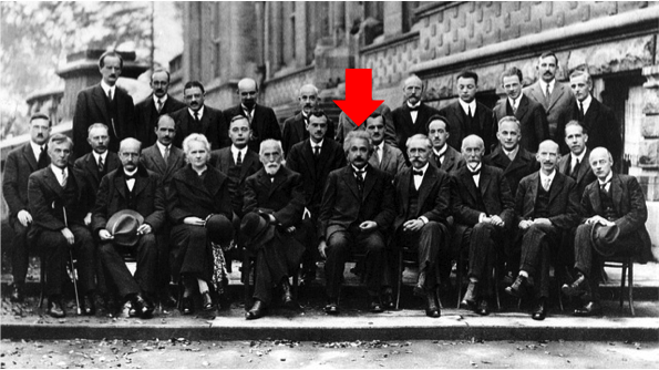
In 1905, five years after Max Planck introduced the Planck relation, where the energy of light E is an integer multiple of the product of the Planck constant h and the light’s frequency v, i.e. E = nhv, Albert Einstein proposed that:

Light, in addition to being a wave, is also a particle of a fixed amount of energy of hv, i.e. the incident electromagnetic radiation is quantised.

A particle of light of energy hv is subsequently called a photon.

Explanation for part 1 of the results

The current produced is proportional to the intensity (brightness) of the incident radiation but independent of its frequency.

If Einstein is correct and light has particle-like behaviour, light intensity can be defined as the rate of photon arrival per unit area. For a fixed value of v, the increase in light intensity is equivalent to the increase in the rate of photon hitting the material at a constant energy of hv per photon. Therefore, when light intensity increases, the amount of ejected electrons reaching Y and flowing in the circuit increases.

For a fixed intensity, increasing the frequency of the incident radiation (i.e., increasing the energy of the incident photons) only increases the kinetic energy of the ejected electrons and not the amount of electrons, as an incident photon, according to Einstein, interacts with an electron by transferring all its energy to the latter (i.e., the energy is not shared by more than one electron). Furthermore, the results are contingent on the incident radiation being above a certain threshold frequency v_o. This led Einstein to establish the following equation:

$hv=\Phi +KE_{max}\; \; \; \; \; \; \; \; 2$

where $\Phi$ is the work function, i.e., the energy needed to overcome the attractive forces between the electron and the nuclei in the material, and KE_max is the maximum kinetic energy of an ejected electron (note that an electron residing deeper in the material has KE<KE_max).

The work function is an intrinsic property of the material (a metal or metalloid) and has a value that varies with different elements.

Question

Why does current increase and reach a saturation value in the second stage of the experiment?

Answer

With the battery connected to the circuit and as the wiper is gradually slid towards T, the potential difference between YX increases. The positively charged Y attracts additional electrons, which previously did not have the proper trajectory to reach it, and the current in the circuit increases. As the wiper slides further away from S, a saturation current is produced because the total number of ejected electrons is dependent only on the incident radiation (assuming that the maximum potential difference across YX is not high enough to ionise any electron at X).

Explanation for part 2 of the results

The absolute value of the stopping voltage is proportional to the frequency of the incident radiation but independent of its intensity.

At the last stage of the experiment, the battery is connected with its positive terminal to X. Electrons leaving X are now subjected to a constant opposing electric force (uniform electric field across XY) that decelerates their motion towards Y. If we assume that the fastest electrons leave X with the same KE_max expressed in eq2 (where $KE_{max}=\frac{1}{2}mv_X^{\;\; 2}=\frac{1}{2}mv_{max}^{\;\; 2}$ ), the difference in kinetic energy between these electrons at X and the same electrons at Y, according to the principle of conservation of energy, must be equal to the energy required to establish the opposing potential difference across XY, i.e. $W=e\Delta V=\frac{1}{2}m\left (v_Y-v_X \right )^2=\frac{1}{2}m\left (v_Y-v_{max} \right )^2$ . Since $v_Y=0$ when no current flows in the circuit, we can expressed the relation between the stopping potential and the maximum kinetic energy of the ejected electrons as:

$eV_{stop}=KE_{max}$

In other words, the higher the kinetic energy of the ejected electrons, the higher the potential needed to stop the current flow. According to eq2, KE_max for a particular cathode is proportional only to v. Therefore, V_stop is proportional to the frequency of the incident radiation but independent of its intensity.

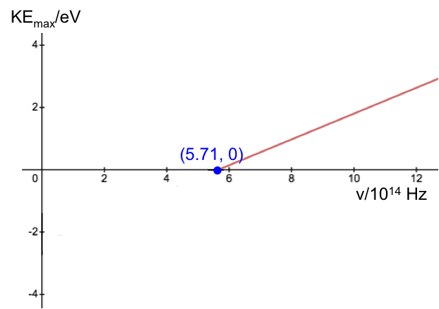
Graphically, we can express parts 1 and 2 of the results as follows:

Explanation for part 3 of the results

The effect is instantaneous, i.e. no time delay between the incidence of light and emission of electrons.

Finally, let’s consider a light of low intensity impinging on the material at X (i.e. light with energy lower than $\Phi$ ). According to the classical wave theory, there would be a time interval between light hitting the material and the emission of an electron. However, current is zero at such an intensity and classical theory fails. Since the emission of electrons does not occur when $E<\Phi$ , and is instantaneous when $E>\Phi$ , light energy must be quantised.

Question

Calculate the Planck constant, the threshold frequency and the work function of sodium using the graph below (1eV = 1.602 x 10^-19 J).

Answer

Rearranging eq2,

$KE_{max}=hv-\Phi$

The value of the work function is given by the vertical intercept, i.e. 2.36 eV.

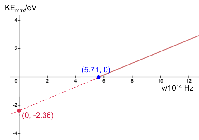
The threshold frequency is the frequency when $KE_{max}=0$ (the horizontal intercept), i.e. 5.71 x 10¹⁴ Hz. The Plank constant is:

$h=\frac{KE_{max}+\Phi}{v}=\frac{2.36\times1.602\times10^{-19}}{5.71\times10^{14}}=6.62\times10^{-34}\, Js$

Next article: de Broglie’s hypothesis

Previous article: Planck’s law

Content page of intermediate quantum chemistry

Content page of intermediate chemistry

Main content page

November 13, 2019November 20, 2024

Planck’s law

Planck’s law is the formula that describes the emission energy-frequency distribution of a black body radiation.

In the late 1800s, scientists tried to offer a mathematical explanation for the frequency profiles of radiation emitted from cavity-in-a-box devices. Lord Rayleigh, a British scientist, used classical physics (in particular, the equipartition theorem where E = kT) to derive a formula called the Rayleigh-Jeans law:

$u(v)=\frac{8\pi v^2kT}{c^3}$

However, the above function only matches the frequency distribution curve at long wavelengths (see below diagram). It diverges when it reaches the ultraviolet range, wrongly implying that an infinite amount of radiation is emitted by the device at short wavelengths, leading to an ‘ultraviolet catastrophe’.

In 1900, Max Planck managed to derive a function that fits the frequency distribution curve very well by assuming that

$E=nhv\; \; \; \; \; \; \; \; 1$

where n is a positive integer, h is a constant called the Planck constant, and v is the frequency of electromagnetic radiation.

This resulted in the Planck distribution function or Planck’s law:

$u(v)dv=\frac{8\pi hv^3kT}{c^3}\frac{1}{e^{kv/kT}-1}dv$

The modern value of h that allows Planck’s law to fit an experimental emission frequency distribution curve very well is 6.626 x 10^-34 J s. This value is known as the Planck constant, which is now the basis for the definition of the kilogramme. Eq1 is called the Planck relation and restricts the energy of electromagnetic radiation to certain discrete values (i.e., electromagnetic energy is quantised). It is this important relation that has led the development of quantum theory.

If you are interested in the complete derivation of Planck’s law, see this article.

Question

What does the positive integer in the Planck relation represent?

Answer

When working on the formula for the frequency distribution curve, Planck assumed that there were n resonating (standing) electromagnetic waves with a particular frequency in the cavity. Einstein, in his experiment, later showed that n also refers to the number of photons, which allows eq1 to be interpreted as the energy of a single photon with the quantised value of hv.

Next article: Photoelectric effect

Previous article: Black body radiation

Content page of intermediate quantum chemistry

Content page of intermediate chemistry

Main content page

November 13, 2019September 25, 2024

Black body radiation

Black body radiation refers to the electromagnetic radiation emitted by a perfect black body, which absorbs all incident radiation and re-emits it as thermal radiation, with a spectrum that depends solely on its temperature.

Electromagnetic radiation falling on an object (body) at a particular temperature can be absorbed, reflected or transmitted by the body. At the same time, a body also emits electromagnetic radiation as part of a conversion of the body’s internal energy to electromagnetic energy.

In fact, a body at thermal equilibrium with its surroundings emits the same amount of radiation of a particular frequency as it absorbs. Otherwise, a body that absorbs radiation better than it emits, or vice versa, will not be in thermal equilibrium with its surroundings. This is known as Kirchhoff’s law of thermal radiation. As the amount of radiation at a particular frequency emitted by a body at a particular temperature varies between different objects, Kirchhoff suggested a reference body to study how matter emits electromagnetic radiation. He hypothesised an ideal body called a black body, which at thermal equilibrium absorbs and emits all frequencies of radiation.

Since then, scientists attempted to design practical models that approximates a black body. Most designs consist of a cavity with a pinhole so small that any electromagnetic radiation that goes into the cavity has very little chance of getting out. Therefore, such a device is considered an ideal absorber of all frequencies of radiation, i.e. one that absorbs more energy via the pinhole than any other body at the same temperature.

In the diagram above, the green arrow represents radiation that enters the cavity though the hole. It is absorbed by the wall of the cavity and re-emitted into the cavity. The re-emitted radiation then gets absorbed and re-emitted so many times within the cavity (red lines) that it attains thermal equilibrium with the cavity wall. Radiation that finally escapes the cavity through the hole (blue line) is passed through a prism to separate the various frequencies, which are measured and analysed. Since the device is deemed an ideal absorber of all frequencies of radiation, it must, according to Kirchhoff’s law of thermal radiation, be an ideal emitter of all frequencies of radiation too.

Enhancements were regularly made to the designs. In 1898, about forty years after Kirchhoff’s suggestion, Otter Lummer and Ferdinand Kurlbaum, both German physicists, constructing a device that significantly improved the measurement of black body radiation. The emitted radiation had the following frequency distribution at various temperatures:

The subsequent challenge was to express the distribution profiles mathematically (see Planck’s law).

Question

With reference to the graph above, cite an example to explain the shift of the peak of an energy-frequency distribution curve to shorter wavelengths at higher temperatures.

Answer

An iron rod glows red when it is heated. This is due to the iron absorbing and re-emitting radiation with wavelength predominantly at the 680-700 nm range.

As it is heated further, it turns white as the iron now absorbs and re-emits radiation over a broader range of wavelengths from 470nm (blue) to 700 nm (red), which combine to form white light. At an even higher temperature, the rod emits blue light because the peak of the distribution curve has narrowed and shifted to the blue wavelength of 470 nm.

Next article: Planck’s law

Previous article: Modern atomic structure

Content page of intermediate quantum chemistry

Content page of intermediate chemistry

Main content page

November 12, 2019November 18, 2024

Reaction Gibbs energy

With reference to eq14 of the previous article, where $\Delta G_{sys}^o=\Delta H_{sys}^o-T\Delta S_{sys}^o$ , we can define the standard reaction Gibbs energy as:

$\Delta G_r^o=\Delta H_r^o-T\Delta S_r^o\; \; \; \; \; \; \; \; 15$

or in general, the reaction Gibbs energy as: $\Delta G_r=\Delta H_r-T\Delta S_r$ .

Furthermore, just as the standard reaction enthalpy is $\Delta H_r^o=\sum_Pv_P(\Delta H_f^o)_P-\sum_Rv_R(\Delta H_f^o)_R$ , and the standard reaction entropy of a system is $\Delta S_r^o=\sum_Pv_P(\Delta S_m^o)_P-\sum_Rv_R(\Delta S_m^o)_R$ , the standard reaction Gibbs energy of a system is:

$\Delta G_r^o=\sum_Pv_P(\Delta G_f^o)_P- \sum_Rv_R(\Delta G_f^o)_R\; \; \; \; \; \; \; \; 16$

where ΔG_f^o is the standard reaction Gibbs energy for the formation of a compound from its elements in their reference states, and v_P and v_R are the stoichiometric coefficients of the products and reactants respectively.

ΔG_r^o, like ΔH_r^o, is computed using energies of formation because we cannot determine the absolute Gibbs energy of a substance (unlike entropy). Even so, the terms ΔG_r^o, ΔH_r^o and ΔS_r^o in eq15 are comparable, as the reference states in $\sum_Pv_P(\Delta G_f^o)_P$ and $\sum_Rv_R(\Delta G_f^o)_R$ as well as those in $\sum_Pv_P(\Delta H_f^o)_P$ and $\sum_Rv_R(\Delta H_f^o)_R$ cancel out when we compute ΔG_r^o and ΔH_r^o respectively (see sections on standard enthalpy change of formation and Hess Law for details).

Combining eq15 and eq16,

$\sum_Pv_P(\Delta G_f^o)_P- \sum_Rv_R(\Delta G_f^o)_R=\Delta H_r^o-T\Delta S_r^o\; \; \; \; \; \; \; \; 17$

Finally, ΔG_r^o is used in the same way as ΔG_sys^o to predict the spontaneity of reactions, where ΔG_r^o < 0 for a spontaneous reaction and ΔG_r^o = 0 when the reaction attains equilibrium.

Question

Calculate the standard combustion Gibbs energy for the reaction $C_2H_6(g)+\frac{7}{2}O_2(g)\rightarrow 2CO_2(g)+3H_2O(l)$ given ΔG_f^o[C₂H₂(g)] = -32.9 kJmol^-1, ΔG_f^o[CO₂(g)] = -394.4 kJmol^-1and ΔG_f^o[H₂O(l)] = -237.2 kJmol^-1.

Answer

Using eq16 and noting that ΔG_f^o[O₂(g)] = 0,

$\Delta G_r^o=(2)(-394.4)+(3)(-237.2)-(-32.9)=-1467.5\, kJmol^{-1}$

Since ΔG_r^o < 0, the reaction is spontaneous.

Previous article: Gibbs energy

Content page of chemical thermodynamics

Content page of intermediate chemistry

Main content page

November 12, 2019September 25, 2024

Gibbs energy

The concept of Gibbs energy was developed by the American scientist Josiah Willard Gibbs in the 1870s.

The change in Gibbs energy of a system is used to measure the spontaneity of reactions at constant temperature and pressure. As mentioned in the previous article, it is defined as:

$\Delta G_{sys}=\Delta H_{sys}-T\Delta S_{sys}\; \; \; \; \; \; \; \; 13$

or under standard conditions:

$\Delta G_{sys}^o=\Delta H_{sys}^o-T\Delta S_{sys}^o\; \; \; \; \; \; \; \; 14$

According to eq12 of the previous article, ΔG_sys^o< 0 for a spontaneous reaction to occur. With reference to eq14 and eq12, the values of ΔH_sys^o, ΔS_sys^oand T influencing the spontaneity of a reaction are summarised as follows:

ΔH_sys^o	ΔS_sys^o	T
–	+	Reaction is spontaneous at any T
–	–	Reaction is spontaneous when $T<\frac{\Delta H_{sys}^o}{\Delta S_{sys}^o}$ , i.e. spontaneity is favoured at low T
+	–	Reaction is not spontaneous at any T
+	+	Reaction is spontaneous when $T>\frac{\Delta H_{sys}^o}{\Delta S_{sys}^o}$ , i.e. spontaneity is favoured at high T

The remarks in the above table is consistent with Le Chatelier’s principle and our knowledge of chemical equilibria, where the increase in temperature of an endothermic and an exothermic reaction shifts the position of equilibrium of a reversible reaction to the right and left respectively, while the decrease in temperature of an endothermic and an exothermic reaction shifts the position of equilibrium to the left and right respectively.

Note that Gibbs energy is previously called Gibbs free energy where the term ‘free’ refers to energy that is “free to do non-pV work”. However in 1988, IUPAC dropped the term to avoid confusion.

Question

Calculate ΔG_sys^ofor the reaction H₂(g) + Cl₂(g) → 2HCl(g) given S_m^o[H₂(g)] = 130.6 JK^-1mol^-1, S_m^o[Cl₂(g)] = 165.0 JK^-1mol^-1, S_m^o[HCl(g)] = 186.8 JK^-1mol^-1and ΔH_sys^o = -184.6 kJmol^-1.

Answer

Using eq14,

$\Delta G_{sys}^o=-184600-(298.15)[(2)(186.8)-(130.6+165.0)]=-207.9\, kJmol^{-1}$

Since ΔG_sys < 0, the reaction is spontaneous.

Next article: Reaction Gibbs energy

Previous article: entropy of the universe

Content page of chemical thermodynamics

Content page of intermediate chemistry

Main content page

November 12, 2019September 25, 2024

Entropy & the 3rd law of thermodynamics

Entropy, denoted by the letter S, is a measure of energy dispersal at a specific temperature. This implies that entropy is a function of temperature, S(T), which allows us to elaborate the concept of entropy using particle motion.

The motion of ions in a solid lattice structure, e.g. NaCl, is restricted to certain vibrational modes at a particular temperature. When we dissolve solid NaCl in water in a beaker, the entropy of the system increases because energy stored in the limited states of the ordered solid ionic lattice structure is dispersed into a large number of energy states of random translational motions of solvated ions throughout the vessel.

By the same logic, when a liquid changes to a gas, particles in the gaseous state move more rapidly and the entropy of the system increases further (as there are even more translational energy states accessible to the substance in the gaseous form). Since the translational energy of a system is temperature-dependent, we’d expect molecular motion and the number of energy states of the system to decrease at a lower system temperature. In fact, a pure substance may form a crystal with one unique state as T → 0 . Such a crystal has an uninterrupted lattice structure and is called a perfect crystal. Furthermore, it is found, through a branch of chemistry known as statistical thermodynamics, that the entropy of a system at T = 0 is zero, i.e. S(0) = 0.

The above phenomenon is summarised in the third law of thermodynamics, which states that

The entropy of a system in a perfect crystalline state is zero as the temperature approaches zero Kelvin.

We can, as a consequence of the 3rd law of thermodynamics, use S(0) = 0 as a reference value to calculate the absolute entropies of substances at any temperature, S(T). Such calculations are often carried out with absolute entropies (or changes in entropies) of systems stated under standard conditions, which are defined as:

1. Temperature: 298.15K (data are sometimes derived at other temperatures)
2. Pressure: 100 kPa or 1 bar
3. Concentration: 1 M
4. State of matter: Each substance is in its normal state (s, l or g) at 100 kPa and 298.15K. For example, the normal state of molecular oxygen at 100 kPa and 298.15K is O₂(g).

The absolute entropy S (or absolute molar entropy S_m) of a substance that is calculated using standard conditions data is given an additional symbol, o, as a superscript to its current symbol, i.e. S^o, with units of JK^-1(or S_m^o, with units of JK^-1mol^-1).

Next article: Standard reaction entropy

Previous article: Entropy

Content page of chemical thermodynamics

Content page of intermediate chemistry

Main content page

November 12, 2019December 8, 2024

Entropy of the universe (Basics)

In chemical thermodynamics, the universe is composed of a system and its surroundings. The system is a part of the universe that is being studied, while its surroundings is the remaining part of the universe, with the two regions separated by a boundary. For example, if we are studying a gaseous reaction in a closed vessel that is in thermal equilibrium with its surroundings, the system is the gas in the vessel, while its surroundings is the space outside the vessel, and the boundary is the thermally conducting vessel walls (see diagram below).

The change in entropy of the universe is given by the sum of the change in entropy of the system and the change in entropy of the surroundings:

$\Delta S_{uni}=\Delta S_{sys}+\Delta S_{sur}\; \; \; \; \; \; \; \; 2$

or under standard conditions:

$\Delta S_{uni}^o=\Delta S_{sys}^o+\Delta S_{sur}^o\; \; \; \; \; \; \; \; 3$

The change in entropy of the universe is sometimes called the total entropy change ΔS_tot^o. However, we are mostly concerned about chemical reactions that are usually defined as occurring within a system, and especially whether such reactions are spontaneous. To determine the spontaneity of a reaction using eq3, we need to know the following facts:

- ΔS_uni^o > 0 for a spontaneous reaction
- ΔS_uni^o = 0 when a reaction reaches equilibrium, where there is no net transfer of heat between a system and its surroundings.

This means that we require, in addition to ΔS_sys^o, the value of ΔS_sur^o, which may not be easily available. To circumvent this problem, we seek a new measure, which can be developed as follows:

For a reaction carried out under standard conditions, ΔS_sys^ois given by eq1 of the previous article, i.e., the standard reaction entropy of the system, ΔS_r^o, while

$\Delta S_{sur}^o=\frac{\Delta H_{sur}^o}{T}\; \; \; \; \; \; \; \; 4$

where T is the temperature of the surroundings, which is equal to the temperature of the system, as the system is at thermal equilibrium with its surroundings.

Although the derivation of eq4 requires knowledge of chemical thermodynamics at the advanced level, we can interpret it by, firstly, noting that the change in enthalpy of the surroundings at constant pressure is equivalent to the amount of heat transferred from the system to the surroundings. We also mentioned in the previous article that an increase in entropy of a system is associated with an increase in number of moles of substances. Rearranging eq4, we get

$T=\frac{\Delta H_{sur}^o}{\Delta S_{sur}^o}\; \; \; \; \; \; \; \; 5$

We can say that the ‘spread’ of a given value of ΔH_sur^o (for a reaction occurring in the surroundings) over a larger increase in the number of moles of substances (i.e. a higher value of ΔS_sur^o) leads to lower energy per particle and hence, lower T.

Having interpreted eq4, let’s consider an exothermic reaction occurring in the system that releases thermal energy that is measured as the change in enthalpy of the system, ΔH_sys^o. Since the system’s vessel walls are thermally conducting, by the theory of conservation of energy, energy transferred from the system to its surroundings increases the energy of the surroundings and decreases the energy of the system, i.e.,

$\Delta H_{sys}^o+\Delta H_{sur}^o=0\; \; \; \; \; \; \; \; 6$

Substituting eq6 in eq4,

$\Delta S_{sur}^o=-\frac{\Delta H_{sys}^o}{T}\; \; \; \; \; \; \; \; 7$

Substituting eq7 in eq3,

$\Delta S_{uni}^o=\Delta S_{sys}^o-\frac{\Delta H_{sys}^o}{T}\; \; \; \; \; \; \; \; 8$

From the previous article, we know that a reaction occurring in a system can result in either positive or negative ΔS_sys^o. Furthermore, we mentioned earlier that:

- ΔS_uni^o > 0 for a spontaneous reaction
- ΔS_uni^o = 0 when a reaction reaches equilibrium, where there is no net transfer of thermal energy between a system and its surroundings.

Therefore, with reference to eq8, if the reaction is exothermic and ΔH_sys^o is large and negative to the extent that ΔS_uni^o > 0, the reaction is spontaneous. For an endothermic reaction to be spontaneous, ΔS_sys^o must be positive enough to compensate for the term $-\frac{\Delta H_{sys}^o}{T}$ .

Substituting eq1 from the previous article and eq7 in eq3,

$\Delta S_{uni}^o=\sum_Pv_P(S_m^o)_P-\sum_Rv_R(S_m^o)_R-\frac{\Delta H_{sys}^o}{T}\; \; \; \; \; \; \; \; 9$

Question

Calculate ΔS_uni for the reaction BaCO₃(s) → BaO(s) + CO₂(g) at 25°C and 1500°C given S_m^o[BaCO₃(s)] = 112.1 JK^-1mol^-1, S_m^o[BaO(s)] = 70.4 JK^-1mol^-1, S_m^o[CO₂(g)] = 213.6 JK^-1mol^-1and ΔH_sys^o = 269.0 kJmol^-1.

Answer

At 25°C, using eq9,

$\Delta S_{uni}^o=70.4+213.6-112.1-\frac{269000}{298.15}=-730.3\,JK^{-1}mol^{-1}$

Since ΔS_uni < 0, the reaction is not spontaneous. This is consistent with the fact that barium carbonate is thermodynamically stable at room temperature.

At 1500°C, if we assume ΔH_sys^oand the standard absolute molar entropies remain unchanged,

$\Delta S_{uni}(1798.15K)=70.4+213.6-112.1-\frac{269000}{1798.15}=22.3\, JK^{-1}mol^{-1}$

The decomposition of barium carbonate becomes spontaneous at this elevated temperature.

Eq8 is a better way to measure the spontaneity of a reaction, as it only requires the calculation of thermodynamic properties of the system. In fact, we can generate a new measure (a new function) in place of ΔS_uni^oto determine the spontaneity of a reaction, starting from:

$\Delta S_{sys}^o-\frac{\Delta H_{sys}^o}{T}>0\; \; \; \; \; \; \; \; 10$

Multiplying eq10 throughout by T,

$T\Delta S_{sys}^o-\Delta H_{sys}^o>0$

$\Delta H_{sys}^o-T\Delta S_{sys}^o<0\; \; \; \; \; \; \; \; 11$

$\Delta G_{sys}^o<0\; \; \; \; \; \; spontaneous\, reaction\; \; \; \; \; \; \; \; 12$

where ΔG_sys^o= ΔH_sys^o – TΔS_sys^o.

We call this function, ΔG_sys^o, the Gibbs energy of the system.

Finally, just as ΔS_uni^o = 0 when a reaction reaches equilibrium, where there is no net transfer of thermal energy between a system and its surroundings, ΔG_sys^o= 0 for a reaction at equilibrium.

Next article: Hund’s rule

Previous article: Pauli exclusion principle

Question

Answer

Next article: Heisenberg’s uncertainty principle

Previous article: Aufbau principle

Question

Answer

Next article: Nuclear spin

Previous article: Hund’s rule

The experiment

Question

Answer

The RESULTS

EXPLANATION OF RESULTS

Question

Answer

Question

Answer

Next article: de Broglie’s hypothesis

Previous article: Planck’s law

Question

Answer

Next article: Photoelectric effect

Previous article: Black body radiation

Question

Answer

Next article: Planck’s law

Previous article: Modern atomic structure

Question

Answer

Previous article: Gibbs energy

Question

Answer

Next article: Reaction Gibbs energy

Previous article: entropy of the universe

Next article: Standard reaction entropy

Previous article: Entropy

Question

Answer

Next article: Gibbs energy

Previous article: Standard reaction entropy