A good quantum number is a label associated with a property of a quantum system that remains constant in time for a given quantum state.
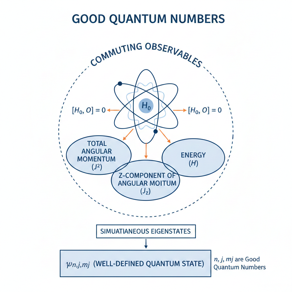
This constancy occurs when the property’s operator commutes with the system’s Hamiltonian
:
To see why, consider the eigenstate of a time-independent Hamiltonian satisfying the time-dependent Schrödinger equation:
Since two commuting operators share a common set of stationary eigenstates, is also an eigenstate of
. When we apply
to the time-evolving state,
where the exponential term factors out in the first equality because it is a scalar.
Therefore, the time-dependent state remains an eigenstate of
with the same eigenvalue
at all times.
Good quantum numbers are preferred in practice because they provide predictability in the time evolution of a quantum system. States labeled by such conserved quantities therefore evolve in a simple and well-understood way. This makes it possible to track the system’s behaviour without continuously redefining the state, which is especially important in spectroscopy. Good quantum numbers also correspond to measurable and reproducible quantities. If a state is an eigenstate of a conserved observable, repeated measurements of that observable yield the same result with certainty. This experimental stability allows states to be prepared, identified and compared reliably. In contrast, observables that are not conserved do not provide fixed labels, since their measured values can change with time even when the system is isolated.
Another reason for preferring good quantum numbers is their close connection to symmetry. Conserved quantities arise from symmetries of the Hamiltonian. Using good quantum numbers therefore exploits the underlying symmetry structure of the system, allowing the Hamiltonian to be block-diagonalised, simplifying both analytical calculations and numerical methods.
For example, a symmetric rotor, such as CH3Cl, has a permanent electric dipole moment along its symmetry axis. In the absence of an external electric field, both the total angular momentum operator and its components
(where
for laboratory axes, or
for the molecular symmetry axis) commute with the Hamiltonian. Therefore,
,
and
are good quantum numbers.

Question
Show that ,
and
commute with the Hamiltonian.
Answer
The Hamiltonian is invariant under a symmetry operation if its expression in different bases related by the symmetry operation is the same. Mathematically,
Multiplying both side by on the right gives
Substituting the definition of a rotation operator into eq320 yields:
where , the angular momentum operator, is the generator of rotations by angle
about axis
.
Expanding the exponential as a Taylor series results in:
Since this equality must hold for any rotation angle, the coefficients for each power of must be equal on both sides. Comparing the 1st order term gives
, or equivalently,
Repeating the above steps using results in
.
To prove that , we substitute
(see this article for derivation), which yields:
Noting that and substituting eq321 into eq322 completes the proof.
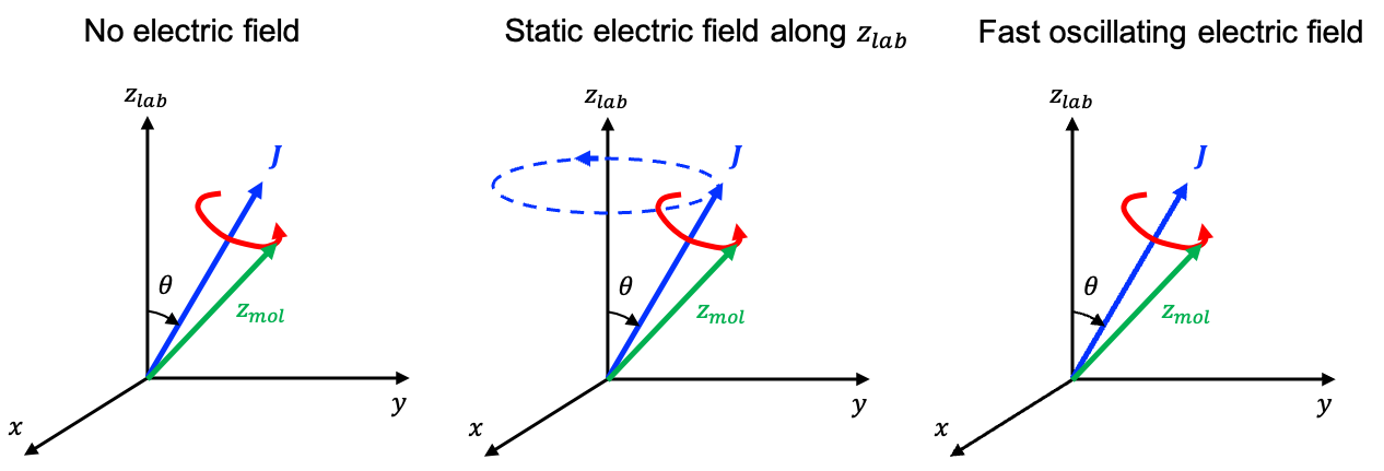
When a static electric field is applied along the laboratory
-axis, it perturbs the molecule such that the Hamiltonian becomes:
where is the unperturbed Hamiltonian and
(see this article for derivation).
(see this article for derivation) still commutes with eq323 because
However, and
no longer commute with eq323. For example,
where (see this article for derivation).
It follows that .
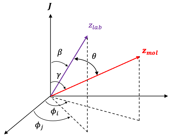
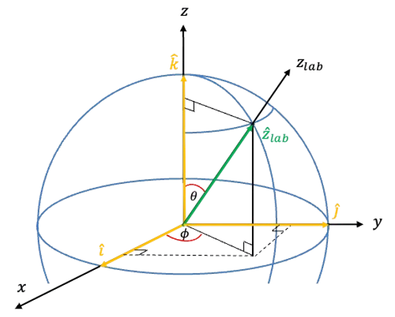
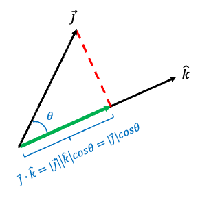
To evalutate the commutation relation between and eq323, we note that
, where
is the angle between the laboratory
-axis and the molecular symmetry axis. Therefore,
where .
Question
Prove that .
Answer
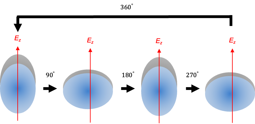
For a symmetric rotor, its orientation is described using Euler angles, where is the angle of rotation of the molecule around its own symmetry axis (see this article for details of the motion of a symmetric rotor in a static electric field). Under a rotation by a small angle
, the wavefunction
transforms as
, which can be expanded in a Taylor series:
In quantum mechanics, such a rotation is described by the rotation operator acting on :
Comparing eq324 and eq325 completes the proof.
Therefore, and
remain as good quantum numbers in the presence of a static electric field, while
is no longer a good quantum number. In general, by repeating the commutation mathematics accordingly, we find that:
|
System |
Good quantum numbers |
|
|
Question
Why are and
good quantum numbers for
-coupling but not
-coupling?
Answer
Russell-Saunders coupling or -coupling occurs in light atoms, where spin-orbit interactions are weak (
). Here, the electrons’ orbital angular momenta couple to form the total orbital angular momentum
separately from their spin angular momenta, which couple to form
, with the total angular momentum given by
. The spin-orbit interaction is a small perturbation to the Hamiltonian, with
, and
,
(see the next article for proof).
On the other hand, -coupling applies when spin-orbit interactions are strong (
), as seen in heavy atoms. In this regime, each electron’s orbital and spin angular momenta couple to form
, and the total angular momentum is
. The corresponding spin-orbit Hamiltonian is
. While
,
and
due to the cross terms (e.g.
).
For more applications of good quantum numbers, see the articles on the Zeeman effect and the Stark effect.