Exchange force is the interaction between particles of a system, as a result of the symmetry of the wavefunction describing the system. This interaction results in a change in the expectation values of inter-particle distances, and hence, a change in energy eigenvalues.
Consider a system of two electrons. The exchange force between electrons is also known as spin correlation. Since the electrons are indistinguishable, the normalised spatial wavefunction can be expressed generally as:
where and
are symmetric spatial wavefunction and anti-symmetric spatial wavefunction respectively of the system of a pair of identical electrons,
and
are orthonormal one-electron wavefunctions, and the notation of
denotes electron 1 in the state
and electron 2 in the state
.
To evaluate the effect of wavefunction symmetry on the expectation values of inter-particle distances, we analyse, for convenience, the average value of the square of the inter-particle distance:
Substitute in the above equation and expanding,
where and
, with
and
.
Applying the Hermitian property of and
for the last two terms of the above equation,
where .
Since the two particles are indistinguishable, . Similarly,
and
. So,
where we have used the logic that because the difference of the terms is zero.
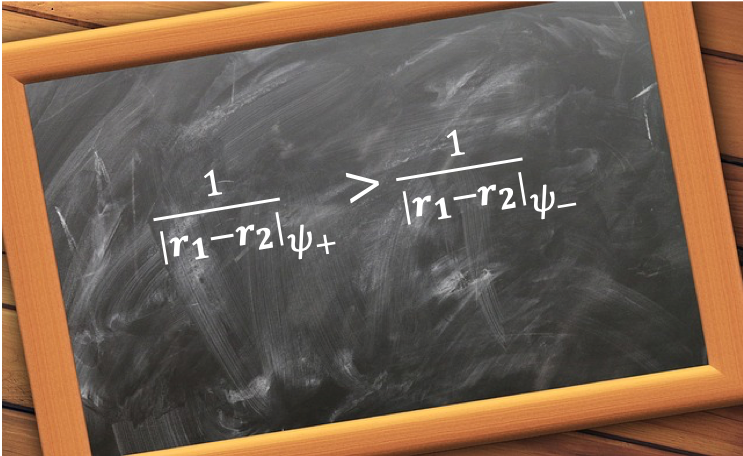
The consequence of eq246 is that , which implies that
The eigenvalues of the Hamiltonian of eq239 are therefore expected to be different for a singlet state and a triplet state because the total wavefunction of the system, according to Pauli’s exclusion principle, must be anti-symmetric with respect to particle exchange.