A p-orbital, defined by the quantum number , is a dumbbell-shaped region of space around the nucleus where an electron is most likely to be found. The letter ”p” is of spectroscopic origin, standing for ‘principal’.
One-electron p-orbital wavefunctions can be expressed using the total wavefunction of a hydrogenic atom:
where
, the radial wavefunction, is the radial component of
.
, the spherical harmonics, is the angular component of
.
are the associated Laguerre polynomials.
are the associated Legendre polynomials.
is the normalisation constant of the radial wavefunction.
is the normalisation constant of the spherical harmonics.
is the principal quantum number, where
is the orbital angular momentum quantum number (also known as azimuthal quantum number), where
and
.
is the magnetic quantum number, where
.
The principal quantum number, , is also called a shell. Since
when
, there are three p-orbitals that are characterised by the set of quantum numbers
of
,
and
in each shell for
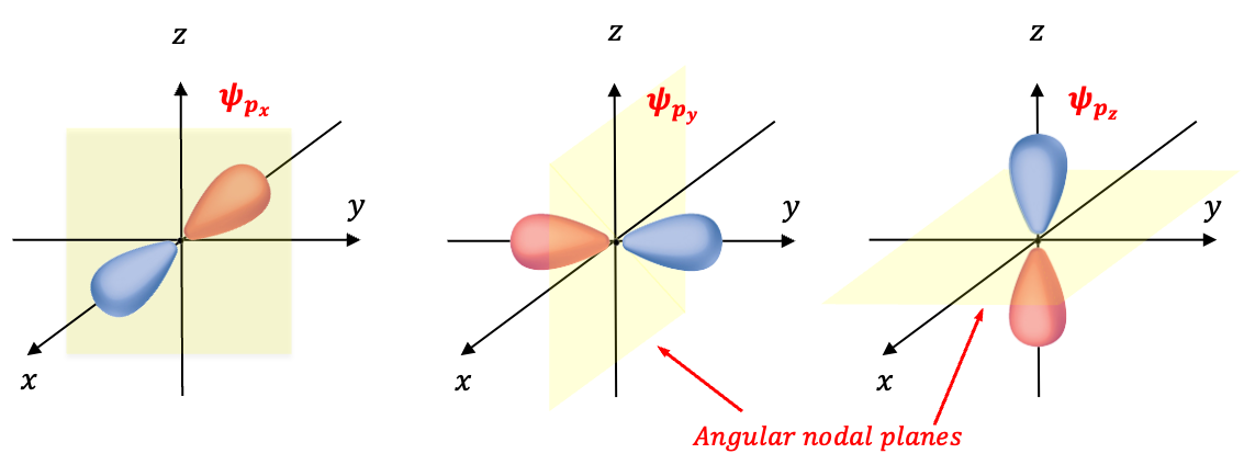
. Each of the three p-orbitals has an angular node. Consider the set
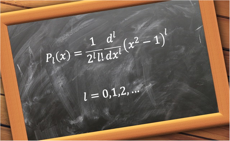
. Substituting these values into the explicit formula for
yields:
where .
Converting from spherical coordinates to Cartesian coordinates, where , gives
Eq474 is known as the orbital. When
, the wavefunction is zero everywhere in the
-plane, which is known as the nodal plane.
For the sets and
, we have
and
, respectively. These two wavefunctions include the factor
, which may complicate calculations when they undergo symmetry operations. Therefore, we take linear combinations of these wavefunctions to form simpler wavefunctions. The first linear combination is
, which normalises to
, or equivalently in Cartesian coordinates:
since .
The second normalised linear combination is , or equivalently,
since .
and
, like
, each have an angular node.

Question
If and
are already normalised, why do we need to normalise a linear combination of them? How do we normalise a linear combination of
and
?
Answer
When forming a linear combination of normalised wavefunctions, the result is not necessarily normalised. Consider a general linear combination , where
and
are coefficients. The normalisation condition for
requires that
, where
represents the volume element in spherical coordinates. Expanding
and noting that
and
are orthonormal, we have
. If
, which is the case for the two linear combinations of
and
,
will not be normalised.
To normalise , we have
or
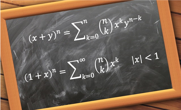
Using (see this article for proof) and some basic trigonometry identities yields
Setting and
gives
.