Advanced Chemistry - Mono Mole

December 7, 2023May 30, 2024

Determinant of a matrix

The determinant is a number associated with an $n\times n$ matrix $A$ . It is defined as

$\vert A\vert=\begin{cases}\vert a_{11}\vert=a_{11}&n=1\\\sum_{j=1}^na_{1j}A_{1j}&n > 1\end{cases}$

where

1. $a_{1j}$ is an element of in the first row of $A$ .
2. $A_{1j}=(-1)^{1+j}M_{1j}^A$ is the cofactor associated with $A$ .
3. $M_{1j}^A$ , the minor of the element $A_{1j}$ , is the determinant of the $n-1 \times n-1$ matrix obtained by removing the $i=1$ row and $j$ -th column of $A$ .

In the case of $n > 1$ , we say that the summation is a cofactor expansion along row 1. For example, the determinant of $A=\begin{pmatrix}a_{11}&a_{12}&a_{13}\\a_{21}&a_{22}&a_{23}\\a_{31}&a_{32}&a_{33}\end{pmatrix}$ is

$\vert A\vert=a_{11}\biggr\vert\begin{matrix}a_{22}&a_{23}\\a_{32}&a_{33}\end{matrix}\biggr\vert-a_{12}\biggr\vert\begin{matrix}a_{21}&a_{23}\\a_{31}&a_{33}\end{matrix}\biggr\vert+a_{13}\biggr\vert\begin{matrix}a_{21}&a_{22}\\a_{31}&a_{32}\end{matrix}\biggr\vert$

For any square matrix, the cofactor expansion along any row and any column results in the same determinant, i.e.

$\vert A\vert=\begin{cases}\vert a_{11}\vert=a_{11}&n=1\\\sum_{i\;or\;j=1}^na_{ij}A_{ij}&n > 1\end{cases}$

To prove this, we begin with the proof that the cofactor expansion along any row results in the same determinant, i.e. $\vert A\vert=\sum_{j=1}^na_{ij}(-1)^{i+j}M_{ij}^A$ for $n > 1$ . Consider a matrix $B$ , which is obtained from $A$ by swapping row $i$ consecutively with rows above it $i-1$ times until it resides in row 1. According to property 8 (see below), we have

$\vert A\vert=(-1)^{i-1}\vert B\vert=(-1)^{i-1}\sum_{j=1}^nb_{1j}(-1)^{1+j}M_{1j}^B\\=(-1)^{i-1}\sum_{j=1}^na_{ij}(-1)^{1+j}M_{ij}^A=\sum_{j=1}^na_{ij}(-1)^{i+j}M_{ij}^A$

According to property 10, $\vert A\vert=\vert A^T\vert$ and therefore, the cofactor expansion along any column also results in the same determinant. This concludes the proof.

In short, to calculate the determinant of an $n > 1$ matrix, we can carry out the cofactor expansion along any row or column. If we expand along a row, we have $\vert A\vert=\sum_{j=1}^na_{ij}A_{ij}$ . We then select any row $i$ to execute the summation. Conversely, if we expand along a column, we get $\vert A\vert=\sum_{i=1}^na_{ij}A_{ij}$ .

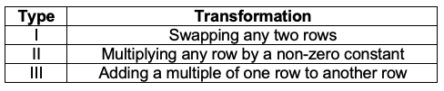
The following are some useful properties of determinants:

1. $\vert I\vert=1$ , where is $I$ the identity matrix. If one of the diagonal elements of $I$ is $k$ , then $\vert I'\vert=k$ .
2. $\vert cI\vert=c^n$
3. If the elements of one of the columns of $A$ are all zero, $\vert A\vert=0$ .
4. If $B$ is obtained from $A$ by multiplying the $p$ -th row of $A$ by $k$ , $\vert B\vert=k\vert A\vert$ .
5. $\vert \varepsilon A\vert=\vert\varepsilon\vert\vert A\vert$
6. $\vert AB\vert=\vert A\vert\vert B\vert$
7. $\vert cA\vert=c^n\vert A\vert$
8. If $B$ is obtained from $A$ by swapping two rows or columns of $A$ , then $\vert B\vert=-\vert A\vert$
9. If two rows or two columns of $A$ are the same, $\vert A\vert=0$ .
10. $\vert A\vert=\vert A^T\vert$
11. The inverse of a matrix exists only if $\vert A\vert\neq 0$ .
12. If $\vert A\vert= 0$ , then $\vert AB\vert=0$ .
13. If $\vert A\vert\neq 0$ , then $\vert A^T\vert\neq 0$ . If $\vert A\vert= 0$ , then $\vert A^T\vert= 0$ .
14. If $A$ is diagonal, then $\vert A\vert= \prod_{i=1}^na_{ii}$ .

Proof of property 1

We shall proof this property by induction.

For $n=1$ ,

$\vert I\vert=\vert 1\vert=1$

For $n=2$ ,

$\sum_{j=1}^2i_{1j}I_{1j}=(1)(-1)^2M_{11}+(0)(-1)^3M_{12}=(1)(-1)^2(1)=1$

Let’s assume that for $n=n-1$ , $\vert I\vert=\sum_{j=1}^{n-1}i_{1j}I_{1j}=1$ . Then for $n=n$ ,

$\vert I\vert=\sum_{j=1}^ni_{1j}I_{1j}=i_{1n}I_{1n}+\sum_{j=1}^{n-1}i_{1j}I_{1j}=(0)I_{1n}+1=1$

We can repeat the above induction logic to prove that $\vert I'\vert=k$ if one of the diagonal elements of $I$ is $k$ .

Proof of property 2

Again, we shall proof this property by induction.

For $n=1$ ,

$\vert cI\vert_1=\vert c\vert=c$

For $n=2$ ,

$\vert cI\vert_2=\sum_{j=1}^2i_{1j}I_{1j}=c(1)(-1)^2M_{11}+c(0)(-1)^3M_{12}=c\vert ci_{22}\vert=c(c)=c^2$

Let’s assume that for $n=n-1$ , we have $\vert cI\vert_{n-1}=c^{n-1}$ . Then for $n=n$ ,

$\vert cI\vert_n=\sum_{j=1}^nci_{1j}I_{1j}=ci_{11}I_{11}+ci_{12}I_{12}+\cdots +ci_{1n}I_{1n}\\=c(1)I_{11}+c(0)I_{12}+\cdots+c(0)I_{1n}=cI_{11}=c\vert cI\vert_{n-1}=cc^{n-1}=c^n$

Proof of property 3

For $n-1$ , where $a_{11}=0$ , we have $\vert A\vert=0$ . For $n>1$ , the definition $\vert A\vert=\sum_{i\;or\;j=1}^na_{ij}A_{ij}$ allows us to sum by row or by column. Suppose we sum by row, we have $\vert A\vert=\sum_{i=1}^na_{ij}A_{ij}$ . Since we are allowed to choose any column $j$ to execute the summation, we can always select the column $j=k$ such that $a_{ik}=0$ . Therefore, $\vert A\vert=0$ if the elements of one of the columns of are all zero.

Proof of property 4

Let’s suppose $B$ is obtained from $A$ by multiplying the $p$ -th row of $A$ by $k$ . If we expand $\vert A\vert$ and $\vert B\vert$ along row $p$ , cofactor $B_{pj}$ is equal to cofactor $A_{pj}$ . Therefore,

$\vert B\vert=\sum_{j=1}^nb_{pj}B_{pj}=\sum_{j=1}^nka_{pj}A_{pj}=k\vert A\vert$

Proof of property 5

For a type I elementary matrix, $\varepsilon A$ transforms $A$ by swapping two rows of $A$ . So, $\vert\varepsilon A\vert=-\vert A\vert$ due to property 8. Since $\varepsilon$ is obtained from $I$ by swapping two rows of $I$ , we have $\vert\varepsilon\vert=-1$ according to property 1 and property 8, which implies that $\vert\varepsilon\vert\vert A\vert=-\vert A\vert$ . Therefore, $\vert\varepsilon A\vert=\vert\varepsilon\vert\vert A\vert$ .

For a type II elementary matrix, $\vert\varepsilon A\vert=k\vert A\vert$ due to property 4 and $\vert\varepsilon\vert\vert A\vert=k\vert A\vert$ because of property 1. So, $\vert\varepsilon A\vert=\vert\varepsilon\vert\vert A\vert$ .

For a type III elementary matrix,

$\vert \varepsilon A\vert=\sum_{j=1}^n(a_{pj}+ka_{qj})A_{pj}=\sum_{j=1}^na_{pj}A_{pj}+k\sum_{j=1}^na_{qj}A_{pj}=\vert A\vert+k\vert B\vert$

$\vert A\vert=\sum_{j=1}^na_{pj}A_{pj}$ is computed by expanding along row $p$ . The equation $\vert B\vert=\sum_{j=1}^na_{qj}A_{pj}$ means that when $\vert B\vert$ is computed by expanding along row $p$ , it has the same cofactor as when $\vert A\vert$ is computed by expanding along row $p$ . This implies that $b_{qj}=a_{qj}$ . Since the definition of the determinant of $B$ is $\vert B\vert=\sum_{j=1}^nb_{pj}B_{pj}$ , which in our case is equivalent to $\vert B\vert=\sum_{j=1}^na_{qj}A_{pj}$ , we have $b_{pj}=a_{qj}$ . Thus $b_{pj}=b_{qj}$ , which according to property 9, gives:

$\vert \varepsilon A\vert=\vert A\vert\;\;\;\;\;\;\;\;5$

Since $\varepsilon =\varepsilon I$ ,

$\vert \varepsilon \vert=\vert \varepsilon I\vert=\vert I\vert=1\;\;\;\;\;\;\;\;6$

according to eq5 and property 1.

Comparing eq5 and eq6, $\vert\varepsilon A\vert=\vert\varepsilon\vert\vert A\vert$ .

Proof of property 6

Case 1

If $A$ is singular, where $\vert A\vert=0$ , then $AB$ is also singular according to property 12. So, $\vert AB\vert=\vert A\vert\vert B\vert$ .

Case 2

If $A$ is non-singular, it can always be expressed as a product of elementary matrices: $A=\varepsilon_1\varepsilon_2\cdots\varepsilon_k$ . So,

$\vert AB\vert=\vert\varepsilon_1(\varepsilon_2\cdots\varepsilon_kB)\vert$

Since property 5 states that $\vert \varepsilon M\vert=\vert\varepsilon\vert\vert M\vert$ ,

$\vert AB\vert=\vert\varepsilon_1\vert\vert\varepsilon_2\cdots\varepsilon_kB\vert=\vert\varepsilon_1\vert\vert\varepsilon_2\vert\vert\varepsilon_3\cdots\varepsilon_kB\vert=\cdots=\vert\varepsilon_1\vert\vert\varepsilon_2\vert\cdots\vert\varepsilon_k\vert\vert B\vert$

Similarly, $\vert A\vert=\vert\varepsilon_1(\varepsilon_2\cdots\varepsilon_k)\vert=\vert\varepsilon_1\vert\vert\varepsilon_2\vert\cdots\vert\varepsilon_k\vert$ . Substitute this in the above equation, $\vert AB\vert=\vert A\vert\vert B\vert$ .

Proof of property 7

Using property 6 and then property 2,

$\vert cA\vert=\vert cIA\vert=\vert cI\vert\vert A\vert=c^n\vert A\vert$

Proof of property 8

We shall proof this property by induction. $n=1$ is the trivial case, where $n$ is the rank of a square matrix.

For $n=2$ , let $A=\begin{pmatrix}a_{11}&a_{12}\\a_{21}&a_{22}\end{pmatrix}$ and $A=\begin{pmatrix}a_{21}&a_{22}\\a_{11}&a_{12}\end{pmatrix}$ , which is obtained from $A$ by swapping two adjacent rows. Furthermore, let $\vert A\vert=\sum_{j=1}^na_{1j}(-1)^{1+j}m_{1j}^A$ and $\vert B\vert=\sum_{j=1}^nb_{1j}(-1)^{1+j}m_{1j}^B$ . Clearly,

$\vert B\vert=a_{21}a_{12}-a_{22}a_{11}=-(a_{11}a_{22}-a_{12}a_{21})=-\vert A\vert$

Let’s assume that for $n=k$ , $\vert B\vert=-\vert A\vert$ when two adjacent rows are swapped. For $n=k+1$ , we have:

Case 1: Suppose that the first row of $A$ is not swapped when making $B$ .

$\vert B\vert=\sum_{j=1}^nb_{1j}(-1)^{1+j}M_{1j}^B=\sum_{j=1}^na_{1j}(-1)^{1+j}M_{1j}^B$

$M_{1j}^B$ is the determinant of a rank $k$ matrix, which is the same as $M_{1j}^A$ except for two adjacent rows being swapped. Therefore, $M_{1j}^B=-M_{1j}^A$ and $\vert B\vert=-\sum_{j=1}^na_{1j}(-1)^{1+j}M_{1j}^A=-\vert A\vert$ .

Case 2: If the first two rows of $A$ are swapped when making $B$ ,

$A=\begin{pmatrix}a_{11}&a_{12}&\cdots&a_{1n}\\a_{21}&a_{22}&\cdots&a_{2n}\\\vdots&\vdots&\ddots&\vdots\\a_{n1}&a_{n2}&\cdots&a_{nn}\end{pmatrix}\;\;\; B=\begin{pmatrix}b_{11}&b_{12}&\cdots&b_{1n}\\b_{21}&b_{22}&\cdots&b_{2n}\\\vdots&\vdots&\ddots&\vdots\\b_{n1}&b_{n2}&\cdots&b_{nn}\end{pmatrix}=\begin{pmatrix}a_{21}&a_{22}&\cdots&a_{2n}\\a_{11}&a_{12}&\cdots&a_{1n}\\\vdots&\vdots&\ddots&\vdots\\a_{n1}&a_{n2}&\cdots&a_{nn}\end{pmatrix}$

We have $\vert A\vert=\sum_{j=1}^na_{1j}(-1)^{1+j}M_{1j}^A$ and $\vert B\vert=\sum_{k=1}^nb_{1k}(-1)^{1+k}M_{1k}^B=\sum_{k=1}^na_{2k}(-1)^{1+k}M_{1k}^B$ . The minors $M_{1j}^A$ and $M_{1k}^B$ can be expressed as

$M_{1j}^A=(1-\delta_{1j})\sum_{k=1}^{j-1}a_{2k}(-1)^{1+k}\vert A_{kj}\vert+\sum_{k=j+1}^na_{2k}(-1)^{k}\vert A_{jk}\vert$

$M_{1k}^B=(1-\delta_{1k})\sum_{j=1}^{k-1}a_{1j}(-1)^{1+j}\vert A_{jk}\vert+\sum_{j=k+1}^na_{1j}(-1)^{j}\vert A_{kj}\vert$

where $A_{kj\;or\;jk}$ is $A$ with the first two rows, and the $k$ -th and $j$ -th columns removed.

Question

Why is each of the minors expressed as two separate sums?

Answer

The minor $M_{1j}^A$ is the determinant of a submatrix of $A$ with the first row and the $j$ -th column of $A$ removed. If $j=1$ , the term with the Kronecker delta disappears and $M_{11}^A=\sum_{k=2}^na_{2k}(-1)^k\vert A_{1k}\vert$ , where $\vert A_{1k}\vert$ is the determinant of $A$ with the first two rows, and the $k$ -th and 1st columns removed. If $1<j<n$ , one of the columns between the 1^st and the last columns of $A$ is removed in forming the submatrix. Therefore, both summations are employed in determining $M_{1j}^A$ , with the first from $k=1$ to $k=j-1$ and the second from $k=j+1$ to $k=n$ . The two summations also apply to the case when $j=n$ . Finally, the same logic can be used to explain the formula for $M_{1k}^B$ . You can validate the formulae of both minors using the example of:

Therefore,

$\vert A\vert=\sum_{j=1}^na_{1j}(-1)^{1+j}\biggr\[(1-\delta_{1j})\sum_{k=1}^{j-1}a_{2k}(-1)^{1+k}\vert A_{kj}\vert+\sum_{k=j+1}^na_{2k}(-1)^{k}\vert A_{jk}\vert\biggr\]$

$\vert B\vert=\sum_{k=1}^na_{2k}(-1)^{1+k}\biggr\[(1-\delta_{1k})\sum_{j=1}^{k-1}a_{1j}(-1)^{1+j}\vert A_{jk}\vert+\sum_{j=k+1}^na_{1j}(-1)^{j}\vert A_{kj}\vert\biggr\]$

For any pair of values of $j$ and $k$ , where $k<j$ , the terms in $\vert A\vert$ are $a_{1j}(-1)^{1+j}\sum_{k=1}^{j-1}a_{2k}(-1)^{1+k}\vert A_{kj}\vert$ , which differ from the terms in $\vert B\vert$ , i.e. $a_{2k}(-1)^{1+k}\sum_{j=k+1}^{n}a_{1j}(-1)^{j}\vert A_{kj}\vert$ , by a factor of -1. Similarly, for any pair of values of $j$ and $k$ , where $k>j$ , the terms in $\vert A\vert$ are $a_{1j}(-1)^{1+j}\sum_{k=j+1}^{n}a_{2k}(-1)^{k}\vert A_{jk}\vert$ , which again differ from the terms in $\vert B\vert$ , i.e. $a_{2k}(-1)^{1+k}\sum_{j=1}^{k-1}a_{1j}(-1)^{1+j}\vert A_{jk}\vert$ , by a factor of -1. Since all terms in $\vert A\vert$ differ from all corresponding terms in $\vert B\vert$ by a factor of -1, $\vert B\vert=-\vert A\vert$ .

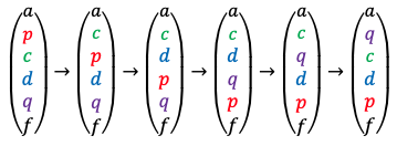
In general, the swapping of any two rows $p$ and $q$ of $A$ , where $1\leq p<q\leq n$ , is equivalent to the swapping of $2(q-p)-1$ adjacent rows of $A$ , with each swap changing $\vert A\vert$ by a factor of -1. Therefore,

$\vert B\vert=(-1)^{2(q-p)-1}\vert A\vert=[(-1)^2]^{p-q}(-1)^{-1}\vert A\vert=-\vert A\vert$

Question

How do we get $2(q-p)-1$ ?

Answer

Firstly, we swap row $p$ consecutively with each row below it until row $q$ is swapped, resulting in $q-p$ swaps. Then, swap the previous row $q$ , which now resides in what was row $q-1$ , consecutively with each row above it until it becomes what used to be row $p$ , resulting in $q-1-p$ swaps. These two actions combined are equivalent to the swapping of $p$ with $q$ , with a total of $2(q-p)-1$ swaps of adjacent rows. The diagram below illustrates an example of the swaps:

Finally, the swapping of any two columns is proven in a similar way.

Proof of property 9

Consider the swapping of two equal rows of $A$ to form $B$ , resulting in $B=A$ and $\vert B\vert=\vert A\vert$ . However, property 8 states that $\vert B\vert=-\vert A\vert$ if any two rows of are swapped. Therefore, $\vert B\vert=\vert A\vert=0$ if two rows of $A$ are equal. The same logic applies to proving $\vert A\vert=0$ if there are two equal columns of $A$ .

Proof of property 10

Case 1: $\vert A\vert=0$

If $\vert A\vert=0$ , then $\vert A^T\vert=0$ according to property 13. So, $\vert A\vert=0=\vert A^T\vert$ .

Case 2: $\vert A\vert\neq 0$

Let’s first consider elementary matrices $\varepsilon$ . A type I elementary matrix is symmetrical about its diagonal, while a type II elementary matrix has one diagonal element equal to $k$ . Therefore, $\varepsilon=\varepsilon^T$ and thus $\vert \varepsilon\vert=\vert\varepsilon^T\vert$ for type I or II elementary matrices. A type III elementary matrix is an identity matrix with one of the non-diagonal elements replaced by a constant $k$ . Therefore, if $\varepsilon$ is a type III elementary matrix, then $\varepsilon^T$ is also one. According to eq6, $\vert\varepsilon\vert=1=\vert\varepsilon^T\vert$ for a type III elementary matrix. Hence, $\vert\varepsilon\vert=\vert\varepsilon^T\vert$ for all elementary matrices.

Next, consider an invertible matrix $A$ , which (as proven in the previous article) can be expressed as $A=\varepsilon_1\varepsilon_2\cdots\varepsilon_k$ . Thus, $A^T=(\varepsilon_1\varepsilon_2\cdots\varepsilon_k)^T=\varepsilon_k^T\cdots\varepsilon_2^T\varepsilon_1^T$ (see Q&A in the proof of property 13). According to property 5,

$\vert A^T\vert=\vert\varepsilon_k^T\cdots\varepsilon_2^T\varepsilon_1^T\vert=\vert\varepsilon_k^T\vert\vert\varepsilon_{k-1}^T\cdots\varepsilon_1^T\vert=\cdots=\vert\varepsilon_k^T\vert\cdots\vert\varepsilon_2^T\vert\vert\varepsilon_1^T\vert=\vert\varepsilon_k\vert\cdots\vert\varepsilon_2\vert\vert\varepsilon_1\vert$

and

$\vert A\vert=\vert\varepsilon_1\varepsilon_2\cdots\varepsilon_k\vert=\vert\varepsilon_1\vert\vert\varepsilon_2\cdots\varepsilon_k\vert=\cdots=\vert\varepsilon_1\vert\vert\varepsilon_2\vert\cdots\vert\varepsilon_k\vert$

Therefore, $\vert A\vert=\vert A^T\vert$ .

Proof of property 11

We have $A^{-1}A=I$ , or in terms of matrix components:

$\sum_{k=1}^n(a^{-1})_{qk}a_{kp}=\delta_{pq}=\frac{\vert A\vert}{\vert A\vert}\delta_{pq}\;\;\;\;\;\;\;\;7$

Consider the matrix $B$ that is obtained from the matrix $A$ by replacing the $q$ -th column of $A$ with the $p$ -th column, i.e. $b_{kq}=a_{kp}$ for $1\leq k\leq n$ and $p\neq q$ . According to property 9, $\vert B\vert=0$ because $B$ has two equal columns. Furthermore, cofactor $B_{kq}$ is equal to cofactor $A_{kq}$ for $1\leq k\leq n$ . Therefore,

$0=\vert B\vert=\sum_{k=1}^nb_{kq}B_{kq}=\sum_{k=1}^na_{kp}A_{kq}\;\;\;\;p\neq q\;\;\;\;\;\;\;\;8$

When $q=p$ , the last summation in eq8 becomes

$\sum_{k=1}^na_{kp}A_{kp}=\vert A\vert\;\;\;\;\;\;\;\;9$

Combining eq8 and eq9, we have $\sum_{k=1}^na_{kp}A_{kq}=\vert A\vert\delta_{pq}$ , which when substituted in eq7 gives:

$\sum_{k=1}^n(a^{-1})_{qk}a_{kp}=\sum_{k=1}^n\frac{A_{kq}}{\vert A\vert}a_{kp}$

Therefore, $(a^{-1})_{qk}=\frac{A_{kq}}{\vert A\vert}$ , which implies that the inverse of a matrix is undefined if $\vert A\vert=0$ . In other words, the inverse of a matrix $A$ is undefined if $\vert A\vert=0$ . We call such a matrix, a singular matrix, and a matrix with an associated inverse, a non-singular matrix.

Proof of property 12

We shall prove by contradiction. According to property 11, $A$ has no inverse if $\vert A\vert=0$ . If $A$ has no inverse and $AB$ has an inverse, then $A\[B(AB)^{-1}\]=I$ . This implies that $A$ has an inverse $A^{-1}$ , where $A^{-1}=B(AB)^{-1}$ , which contradicts the initial assumption that $A$ has no inverse. Therefore, if $A$ has no inverse, then $AB$ must also have no inverse.

Proof of property 13

Question

Show that $(ABC\cdots)^T=\cdots C^TB^TA^T$ .

Answer

$(AB)^T=B^TA^T$ because

$(AB)^T_{ij}=(AB)_{ji}=\sum_{k=1}^na_{jk}b_{ki}=\sum_{k=1}^n(A^T)_{kj}(B^T)_{ik}\\=\sum_{k=1}^n(B^T)_{ik}(A^T)_{kj}=(B^TA^T)_{ij}$

$(ABC)^T=C^TB^TA^T$ because

$(ABC)^T_{ij}=(ABC)_{ji}=\sum_{l=1}^n\sum_{k=1}^na_{jk}b_{kl}c_{li}=\sum_{l=1}^n\sum_{k=1}^n(A^T)_{kj}(B^T)_{lk}(C^T)_{il}\\=\sum_{l=1}^n\sum_{k=1}^n(C^T)_{il}(B^T)_{lk}(A^T)_{kj}=(C^TB^TA^T)_{ij}$

which can be extended to $(ABC\cdots)^T=\cdots C^TB^TA^T$ .

Using the identity in the above Q&A, $(A^{-1})^TA^T=(AA^{-1})^T$ . If $A$ is invertible, then $(A^{-1})^TA^T=(AA^{-1})^T=I=(A^{-1}A)^T=A^T(A^{-1})^T$ . This implies that $(A^{-1})^T$ is the inverse of $A^T$ and therefore that $A^T$ is invertible if $A$ is invertible.

The last part shall be proven by contradiction. Suppose $A$ is singular and $A^T$ is non-singular, there would be a matrix $B$ such that $BA^T=I$ , Furthermore, $I=I^T=(BA^T)^T=AB^T$ , which implies that $B^T=A^{-1}$ . This contradicts our initial assumption that $A$ is singular. Therefore, if $A$ is singular, $A^T$ must also be singular.

Proof of property 14

We shall proof this property by induction. For $n=2$ ,

$\vert A\vert=a_{11}a_{22}=\prod_{i=1}^2a_{ii}$

Let’s assume that $\vert A\vert=\prod_{i=1}^na_{ii}$ for $n=n$ . Then for $n=n+1$ , the cofactor expansion along the first row is

$\vert A\vert=a_{11}\begin{vmatrix}a_{22}&0&\cdots&0\\0&a_{33}&\cdots&0\\0&0&\ddots&\vdots\\0&0&\cdots&a_{n+1,n+1}\end{vmatrix}=a_{11}\prod_{i=2}^{n+1}a_{ii}=\prod_{i=1}^{n+1}a_{ii}$

Next article: Schur’s first lemma

Previous article: Elementary row operation and elementary matrix

Content page of group theory

Content page of advanced chemistry

Main content page

December 7, 2023April 20, 2024

Schur’s first lemma

Schur’s first lemma states that a non-zero matrix that commutes with all matrices of an irreducible representation of a group is a multiple of the identity matrix.

The proof of Schur’s first lemma involves the following steps:

1. Consider a representation of a group $G$ , i.e. $\Gamma=\{A_1,A_2,\cdots,A_{\vert G\vert}\}$ , where each element of $\Gamma$ is an $n\times n$ matrix, which can be regarded as a unitary matrix $U$ according to a previous article.
2. Proof that a Hermitian matrix $H$ that commutes with the irreducible representation element $A_{\alpha}$ , where $\alpha=1,2,\cdots,\vert G\vert$ , is a constant multiple of the identity matrix.
3. Infer from step 2 that any arbitrary non-zero matrix $M$ that commutes with the irreducible representation element $A_{\alpha}$ is a multiple of the identity matrix.

Step 1 is self-explanatory. For step 2, we begin with a Hermitian matrix $H$ that commutes with $A_{\alpha}$ :

$HA_{\alpha}=A_{\alpha}H$

Multiplying the above equation on the left and right by $U^{-1}$ and $U$ respectively,

$U^{-1}HA_{\alpha}U=U^{-1}A_{\alpha}HU$

Since $UU^{-1}=I$

$U^{-1}HUU^{-1}A_{\alpha}U=U^{-1}A_{\alpha}UU^{-1}HU$

$U^{-1}HU\tilde A_{\alpha}=\tilde A_{\alpha}U^{-1}HU$

where $\tilde A_{\alpha}=U^{-1}A_{\alpha}U$ .

Question

Show that $\tilde A_{\alpha}$ is also a representation of $G$ .

Answer

If $\tilde A_{\alpha}$ is also a representation of $G$ , its elements must multiply according to the multiplication table of $G=\{A_1,A_2,\cdots,A_{\vert G\vert}\}$ . Since $\tilde A_{\alpha}=U^{-1}A_{\alpha}U$ , we have

$\tilde A_{i}\tilde A_j=(U^{-1}A_iU)(U^{-1}A_jU)=U^{-1}A_iA_jU=U^{-1}A_kU=\tilde A_k$

The third equality ensures that the closure property of $G$ is satisfied for $A_{\alpha}$ and hence $\tilde A_{\alpha}$ . In other words, the elements of $G=\{\tilde A_1,\tilde A_2,\cdots,\tilde A_{\vert G\vert}\}$ multiply according to the multiplication table of $G=\{A_1,A_2,\cdots,A_{\vert G\vert}\}$ .

As a Hermitian matrix can undergo a similarity transformation by a unitary matrix to give another Hermitian matrix $D$ which is diagonal, i.e. $U^{-1}HU=D$ , we have

$D\tilde A_{\alpha}=\tilde A_{\alpha}D$

Rewriting $D\tilde A_{\alpha}=\tilde A_{\alpha}D$ in terms of its matrix elements, we have $(D\tilde A_{\alpha})_{mn}=(\tilde A_{\alpha}D)_{mn}$ or $D_{mm}(\tilde A_{\alpha})_{mn}=(\tilde A_{\alpha})_{mn}D_{nn}$ , which can be rearranged to

$(\tilde A_{\alpha})_{mn}(D_{mm}-D_{nn})=0$

Consider the following cases for the above equation:

Case 1: All diagonal elements of $D$ are distinct, i.e. $D_{mm}\neq D_{nn}$ if $m\neq n$ .

We have $(\tilde A_{\alpha})_{mn}=0$ for $m\neq n$ , which means that all off-diagonal elements of $\tilde A_{\alpha}$ are zero. In other words, $\tilde A_{\alpha}$ is an element of a reducible representation that is a direct sum of $n$ elements of one-dimensional matrix representations. Furthermore, the definition of a reducible representation implies that $A_{\alpha}$ is also an element of a reducible representation of $G$ because $\tilde A_{\alpha}=U^{-1}A_{\alpha}U$ .

Case 2: All diagonal elements of $D$ are equal, i.e. $D_{mm}=D_{nn}\;\forall\; m,n$ .

$(\tilde A_{\alpha})_{mn}$ can be any finite number, and consequently $\tilde A_{\alpha}$ may be either an element of a reducible or an irreducible representation. However, the diagonal matrix $D$ must be a multiple of the identity matrix if $D_{mm}=D_{nn}\;\forall\; m,n$ .

Case 3: Some but not all diagonal elements of $D$ are equal.

Instead of considering all possible permutations of equal and unequal diagonal entries in $D$ , we rearrange the columns of $U$ such that equal diagonal entries of $D$ are in adjacent columns of $D$ . This is always possible as the order of the columns of $U$ corresponds to the order of the diagonal entries in $D$ (see this article). Let’s suppose the first $i$ diagonal entries are the same, while the rest are distinct, i.e. $D_{11}=D_{22}=\cdots=D_{ii}\neq D_{i+1,i+1}\neq\cdots\neq D_{nn}$ . With reference to Case 1 and Case 2, $\tilde A_{\alpha}$ must be an element of a reducible representation with the block diagonal form:

$\tilde A_{\alpha}\begin{pmatrix}X&0\\0&Y\end{pmatrix}$

For example, if $D_{11}=D_{22}\neq D_{33}\neq D_{44}$ in the following $4\times 4$ matrix,

then $(\tilde A_1)_{12},(\tilde A_1)_{21}$ can be any finite number, while all other off-diagonal elements are zero.

Combining all three cases, if $\tilde A_{\alpha}$ is an irreducible representation, the diagonal matrix $D$ must be a multiple of the identity matrix. Since $D\tilde A_{\alpha}=\tilde A_{\alpha}D$ , where $D$ is Hermitian, we have proven step 2.

For the last step, let’s consider an arbitrary non-zero matrix $M$ that commutes with $A_{\alpha}$ :

$MA_{\alpha}=A_{\alpha}M\;\;or\;\;A_{\alpha}^{\dagger}M^{\dagger}=M^{\dagger}A_{\alpha}^{\dagger}$

Since $A_{\alpha}$ is unitary, $A_{\alpha}^{\dagger}=A_{\alpha}^{-1}$ and so $A_{\alpha}^{-1}M^{\dagger}=M^{\dagger}A_{\alpha}^{-1}$ , which when multiplied from the left and right by $A_{\alpha}$ gives $M^{\dagger}A_{\alpha}=A_{\alpha}M^{\dagger}$ . This implies that if $M$ commutes with $A_{\alpha}$ , then $M^{\dagger}$ also commutes with $A_{\alpha}$ .

Question

i) Show that if $M$ and $M^{\dagger}$ commutes with $A_{\alpha}$ , then any linear combination of $M$ and $M^{\dagger}$ also commutes with $A_{\alpha}$ .
ii) Show that the linear combinations $H_1=M+M^{\dagger}$ and $H_2=iM-M^{\dagger}$ are Hermitian.
iii) Show that $M=\frac{H_1-iH_2}{2}$ .

Answer

$(aM+bM^{\dagger})A_{\alpha}=aMA_{\alpha}+bM^{\dagger}A_{\alpha}=aA_{\alpha}M+bA_{\alpha}M^{\dagger}=A_{\alpha}(aM+bM^{\dagger})$

ii)

$H_1^{\dagger}=(M+M^{\dagger})^{\dagger}=M^{\dagger}+M=H_1$
$H_2^{\dagger}=(iM-iM^{\dagger})^{\dagger}=-iM^{\dagger}+iM=H_2$
iii) Substitute $H_1=M+M^{\dagger}$ and $H_2=iM-iM^{\dagger}$ in $\frac{H_1-iH_2}{2}$ , we get $M$ .

With reference to step 2, $H_1$ must be a constant multiple of the identity matrix and so must $H_2$ . Therefore, $\frac{H_1-iH_2}{2}$ is also a constant multiple of the identity matrix. This concludes that proof of Schur’s first lemma, which together with Schur’s second lemma, is used to proof the great orthogonality theorem.

Next article: Schur’s second lemma

Previous article: determinant of a matrix