Advanced Chemistry - Mono Mole

December 7, 2022July 14, 2025

Gram-Schmidt Process

The Gram-Schmidt process is a mathematical technique for orthogonalising a set of nonorthogonal vectors.

Consider two linearly independent nonorthogonal vectors $\boldsymbol{\mathit{ x}}_1$ and $\boldsymbol{\mathit{ x}}_2$ of the Hermitian operator $\hat O$ :

$\hat O\boldsymbol{\mathit{ x}}_1=a\boldsymbol{\mathit{ x}}_1$

$\hat O\boldsymbol{\mathit{ x}}_2=a\boldsymbol{\mathit{ x}}_2$

where $a$ is the degenerate eigenvalue corresponding to $\boldsymbol{\mathit{ x}}_1$ and $\boldsymbol{\mathit{ x}}_2$ .

Let $\boldsymbol{\mathit{ x}}_1=\boldsymbol{\mathit{ x}}_1^{'}$ . With reference to the diagram above, $\vert\boldsymbol{\mathit{ x}}_{2p}\vert=\vert\boldsymbol{\mathit{ x}}_2\vert cos\theta=\boldsymbol{\mathit{ x}}_2\cdot\frac{\boldsymbol{\mathit{ x}}_1^{'}}{\vert\boldsymbol{\mathit{ x}}_1^{'}\vert}$ , where we have used the fact that the magnitude of the unit vector $\frac{\boldsymbol{\mathit{ x}}_1^{'}}{\vert\boldsymbol{\mathit{ x}}_1^{'}\vert}$ is 1 in the second equality. Furthermore, $\boldsymbol{\mathit{ x}}_{2p}=\vert\boldsymbol{\mathit{ x}}_{2p}\vert \frac{\boldsymbol{\mathit{ x}}_1^{'}}{\vert\boldsymbol{\mathit{ x}}_1^{'}\vert}$ ; that is, the vector $\boldsymbol{\mathit{ x}}_{2p}$ is a multiple of the unit vector $\frac{\boldsymbol{\mathit{ x}}_1^{'}}{\vert\boldsymbol{\mathit{ x}}_1^{'}\vert}$ , with the multiple being $\vert\boldsymbol{\mathit{ x}}_{2p}\vert$ . Therefore,

$\boldsymbol{\mathit{ x}}_2^{'}=\boldsymbol{\mathit{ x}}_2-\boldsymbol{\mathit{ x}}_{2p}=\boldsymbol{\mathit{ x}}_2-\vert\boldsymbol{\mathit{ x}}_{2p}\vert\frac{\boldsymbol{\mathit{ x}}_1^{'}}{\vert\boldsymbol{\mathit{ x}}_1^{'}\vert}=\boldsymbol{\mathit{ x}}_2-\left(\boldsymbol{\mathit{ x}}_2\cdot\frac{\boldsymbol{\mathit{ x}}_1^{'}}{\vert\boldsymbol{\mathit{ x}}_1^{'}\vert}\right)\frac{\boldsymbol{\mathit{ x}}_1^{'}}{\vert\boldsymbol{\mathit{ x}}_1^{'}\vert}$ $=\boldsymbol{\mathit{ x}}_2-\frac{\boldsymbol{\boldsymbol{\mathit{ x}}_2\cdot\mathit{ x}}_1^{'}}{\vert\boldsymbol{\mathit{ x}}_1^{'}\vert^2}\boldsymbol{\mathit{ x}}_1^{'}=\boldsymbol{\mathit{ x}}_2-\frac{\boldsymbol{\boldsymbol{\mathit{ x}}_2\cdot\mathit{ x}}_1^{'}}{\boldsymbol{\mathit{ x}}_1^{'}\cdot\boldsymbol{\mathit{ x}}_1^{'}}\boldsymbol{\mathit{ x}}_1^{'}\;\;\;\;\;\;\;\;(111)$
$\boldsymbol{\mathit{ x}}_2^{'}$ is a component of $\boldsymbol{\mathit{ x}}_2$ , which is orthogonal to $\boldsymbol{\mathit{ x}}_1^{'}$ . The eigenvalue of $\boldsymbol{\mathit{ x}}_2^{'}$ is unchanged versus that of $\boldsymbol{\mathit{ x}}_2$ because

$\hat O\left(\boldsymbol{\mathit{ x}}_2-\frac{\boldsymbol{\boldsymbol{\mathit{ x}}_2\cdot\mathit{ x}}_1^{'}}{\boldsymbol{\mathit{ x}}_1^{'}\cdot\boldsymbol{\mathit{ x}}_1^{'}}\boldsymbol{\mathit{ x}}_1^{'}\right)=\hat O\boldsymbol{\mathit{ x}}_2-\frac{\boldsymbol{\boldsymbol{\mathit{ x}}_2\cdot\mathit{ x}}_1^{'}}{\boldsymbol{\mathit{ x}}_1^{'}\cdot\boldsymbol{\mathit{ x}}_1^{'}}\hat O\boldsymbol{\mathit{ x}}_1^{'}=a\left(\boldsymbol{\mathit{ x}}_2-\frac{\boldsymbol{\boldsymbol{\mathit{ x}}_2\cdot\mathit{ x}}_1^{'}}{\boldsymbol{\mathit{ x}}_1^{'}\cdot\boldsymbol{\mathit{ x}}_1^{'}}\boldsymbol{\mathit{ x}}_1^{'}\right)$

In the presence of a third linearly independent vector $\boldsymbol{\mathit{ x}}_3$ that is nonorthogonal to $\boldsymbol{\mathit{ x}}_1$ and $\boldsymbol{\mathit{ x}}_2$ (where $\hat O\boldsymbol{\mathit{ x}}_3=a\boldsymbol{\mathit{ x}}_3$ ), the vector $\boldsymbol{\mathit{ x}}_{3a}^{'}$ that is orthogonal to $\boldsymbol{\mathit{ x}}_{1}^{'}$ is $\boldsymbol{\mathit{ x}}_{3a}^{'}=\boldsymbol{\mathit{ x}}_3-\frac{\boldsymbol{\boldsymbol{\mathit{ x}}_3\cdot\mathit{ x}}_1^{'}}{\boldsymbol{\mathit{ x}}_1^{'}\cdot\boldsymbol{\mathit{ x}}_1^{'}}\boldsymbol{\mathit{ x}}_1^{'}$ (c.f. eq111). To determine the component of $\boldsymbol{\mathit{ x}}_3$ that is orthogonal to both $\boldsymbol{\mathit{ x}}_{1}^{'}$ and $\boldsymbol{\mathit{ x}}_{2}^{'}$ , let $\boldsymbol{\mathit{ x}}_{3}^{'}$ be the component of $\boldsymbol{\mathit{ x}}_{3a}^{'}$ that is orthogonal to $\boldsymbol{\mathit{ x}}_{2}^{'}$ :
$\boldsymbol{\mathit{ x}}_3^{'}=\boldsymbol{\mathit{ x}}_{3a}^{'}-\frac{\boldsymbol{\boldsymbol{\mathit{ x}}_{3a}^{'}\cdot\mathit{ x}}_2^{'}}{\boldsymbol{\mathit{ x}}_2^{'}\cdot\boldsymbol{\mathit{ x}}_2^{'}}\boldsymbol{\mathit{ x}}_2^{'}$

We can immediately see that $\boldsymbol{\mathit{ x}}_{3}^{'}$ is orthogonal to both $\boldsymbol{\mathit{ x}}_{1}^{'}$ and $\boldsymbol{\mathit{ x}}_{2}^{'}$ because it is sum of two vectors $\boldsymbol{\mathit{ x}}_{3a}^{'}$ and $\boldsymbol{\mathit{ x}}_{2}^{'}$ , each of which is orthogonal to $\boldsymbol{\mathit{ x}}_{1}^{'}$ (and hence the dot product $\boldsymbol{\mathit{ x}}_{3}^{'}\cdot\boldsymbol{\mathit{ x}}_{1}^{'}$ is zero). Substituting $\boldsymbol{\mathit{ x}}_{3a}^{'}=\boldsymbol{\mathit{ x}}_3-\frac{\boldsymbol{\boldsymbol{\mathit{ x}}_3\cdot\mathit{ x}}_1^{'}}{\boldsymbol{\mathit{ x}}_1^{'}\cdot\boldsymbol{\mathit{ x}}_1^{'}}\boldsymbol{\mathit{ x}}_1^{'}$ in the above equation, noting that $\frac{\boldsymbol{\boldsymbol{\mathit{ x}}_3\cdot\mathit{ x}}_1^{'}}{\boldsymbol{\mathit{ x}}_1\cdot\boldsymbol{\mathit{ x}}_1^{'}}$ and $\frac{\boldsymbol{\mathit{ x}}_2^{'}}{\boldsymbol{\mathit{ x}}_2^{'}\cdot\boldsymbol{\mathit{ x}}_2^{'}}$ are scalars and that $\boldsymbol{\mathit{ x}}_1^{'}\cdot\boldsymbol{\mathit{ x}}_2^{'}=0$ , we have

$\boldsymbol{\mathit{ x}}_3^{'}=\boldsymbol{\mathit{ x}}_{3}-\frac{\boldsymbol{\boldsymbol{\mathit{ x}}_{3}\cdot\mathit{ x}}_1^{'}}{\boldsymbol{\mathit{ x}}_1\cdot\boldsymbol{\mathit{ x}}_1^{'}}\boldsymbol{\mathit{ x}}_1^{'}-\frac{\boldsymbol{\boldsymbol{\mathit{ x}}_{3}\cdot\mathit{ x}}_2^{'}}{\boldsymbol{\mathit{ x}}_2^{'}\cdot\boldsymbol{\mathit{ x}}_2^{'}}\boldsymbol{\mathit{ x}}_2^{'}\;\;\;\;\;\;\;\;(112)$

Therefore, for a set of three linearly independent nonorthogonal vectors $\{\boldsymbol{\mathit{ x}}_1,\boldsymbol{\mathit{ x}}_2,\boldsymbol{\mathit{ x}}_3\}$ , the transformed set of vectors, which are orthogonal to one another, is $\{\boldsymbol{\mathit{ x}}_1^{'},\boldsymbol{\mathit{ x}}_2^{'},\boldsymbol{\mathit{ x}}_3^{'}\}$ , where

$\boldsymbol{\mathit{ x}}_1^{'}=\boldsymbol{\mathit{ x}}_{1}$

$\boldsymbol{\mathit{ x}}_2^{'}=\boldsymbol{\mathit{ x}}_{2}-\frac{\boldsymbol{\boldsymbol{\mathit{ x}}_{2}\cdot\mathit{ x}}_1^{'}}{\boldsymbol{\mathit{ x}}_1^{'}\cdot\boldsymbol{\mathit{ x}}_1^{'}}\boldsymbol{\mathit{ x}}_1^{'}$

For a set of linearly independent nonorthogonal vectors $\{\boldsymbol{\mathit{ x}}_1,\boldsymbol{\mathit{ x}}_2,\cdots,\boldsymbol{\mathit{ x}}_k\}$ , the transformed set of vectors, which are orthogonal to one another, is $\{\boldsymbol{\mathit{ x}}_1^{'},\boldsymbol{\mathit{ x}}_2^{/},\cdots,\boldsymbol{\mathit{ x}}_k^{'}\}$ with the k-th transformed vector as

$\boldsymbol{\mathit{ x}}_k^{'}=\boldsymbol{\mathit{ x}}_{k}-\frac{\boldsymbol{\boldsymbol{\mathit{ x}}_{k}\cdot\mathit{ x}}_1^{'}}{\boldsymbol{\mathit{ x}}_1\cdot\boldsymbol{\mathit{ x}}_1^{'}}\boldsymbol{\mathit{ x}}_1^{'}-\frac{\boldsymbol{\boldsymbol{\mathit{ x}}_{k}\cdot\mathit{ x}}_2^{'}}{\boldsymbol{\mathit{ x}}_2^{'}\cdot\boldsymbol{\mathit{ x}}_2^{'}}\boldsymbol{\mathit{ x}}_2^{'}-\cdots-\frac{\boldsymbol{\boldsymbol{\mathit{ x}}_{k}\cdot\mathit{ x}}_{k-1}^{'}}{\boldsymbol{\mathit{ x}}_{k-1}^{'}\cdot\boldsymbol{\mathit{ x}}_{k-1}^{'}}\boldsymbol{\mathit{ x}}_{k-1}^{'}$

The corresponding orthonormal vectors are $\boldsymbol{\mathit{ e}}_1=\frac{\boldsymbol{\mathit{ x}}_1^{'}}{\vert\boldsymbol{\mathit{ x}}_1^{'}\vert}$ , $\boldsymbol{\mathit{ e}}_2=\frac{\boldsymbol{\mathit{ x}}_2^{'}}{\vert\boldsymbol{\mathit{ x}}_2^{'}\vert}$ , … , $\boldsymbol{\mathit{ e}}_k=\frac{\boldsymbol{\mathit{ x}}_k^{'}}{\vert\boldsymbol{\mathit{ x}}_k^{'}\vert}$ .

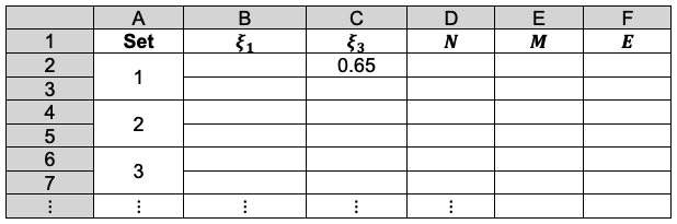
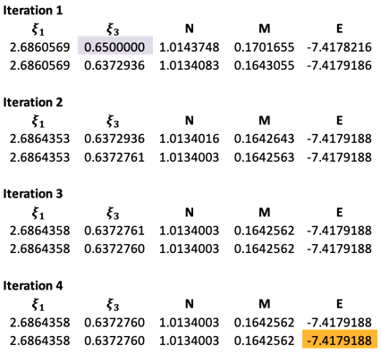
An example of the application of the Gram-Schmidt process is the orthogonalisation of nonorthogonal Slater-type orbitals in the Hartree-Fock method.

Next article: Spin-orbital

Previous article: Canonical Hartree-Fock equations

Content page of computational chemistry

Content page of advanced chemistry

Main content page

December 7, 2022December 27, 2024

Spin-orbital

A spin-orbital $\phi(x)$ expresses the state of an electron as a complete wavefunction, which comprises of a spatial component and a spin component.

It is defined as

$\phi(x)=\left\{\begin{matrix}\chi(\boldsymbol{\mathit{ r}})\alpha(\omega)\\\chi(\boldsymbol{\mathit{ r}})\beta(\omega) \end{matrix}\right.$

where $x$ is a composite coordinate consisting of three spatial coordinates $\boldsymbol{\mathit{ r}}$ and one spin coordinate $\omega$ , while $\alpha$ and $\beta$ are spin wavefunctions describing the two possible spin states of an electron.

In the derivation of the canonical Hartree-Fock equations, $\phi_t^{'}(x)=\chi_t^{'}(\boldsymbol{\mathit{ r}})\sigma(\omega)$ , where $\sigma=\alpha\;or\;\beta$ . When we substitute the spin-orbitals in their explicit forms into eq109, we have

$\biggr[\left(-\frac{1}{2}\nabla^2-\frac{Z}{r}\right)+\sum_{t\neq r}\int\int\chi_t^{'*}(\boldsymbol{\mathit{ r}}')\sigma^*(\omega^{'}) \frac{(1-P_{rt})\chi_t^{'}(\boldsymbol{\mathit{ r}}')\sigma(\omega^{'})}{\vert\boldsymbol{\mathit{ r}}-\boldsymbol{\mathit{ r}}'\vert}d\boldsymbol{\mathit{ r}}'d\omega'\biggr]$ $\chi_r^{'}(\boldsymbol{\mathit{ r}})\sigma(\omega)=\lambda_r^{'}\chi_r^{'}(\boldsymbol{\mathit{ r}}')\sigma(\omega^{'})$
Multiplying throughout by $\sigma^{'}(\omega)$ and integrating with respect to the spin coordinates, while noting that $\int\sigma^{'}(\omega)\sigma(\omega)=\delta_{\sigma^{'}\sigma}$ because of spin orthogonality, we have

$\biggr[\left(-\frac{1}{2}\nabla^2-\frac{Z}{r}\right)+\sum_{t\neq r}\int\chi_t^{'*}(\boldsymbol{\mathit{ r}}')\frac{(1-P_{rt})\chi_t^{'}(\boldsymbol{\mathit{ r}}')}{\vert\boldsymbol{\mathit{ r}}-\boldsymbol{\mathit{ r}}'\vert}d\boldsymbol{\mathit{ r}}'\biggr]\chi_r^{'}(\boldsymbol{\mathit{ r}})=\lambda_r^{'}\chi_r^{'}(\boldsymbol{\mathit{ r}}')$

Question

Why are the spin components of the total wavefunction orthogonal?

Answer

From the article on Hermitian operators, we know that two eigenfunctions of a Hermitian operator that correspond to different eigenvalues are orthogonal. Since the spin components of the total wavefunction $\alpha$ and $\beta$ correspond to different eigenvalues of the spin Hermitian operator $\hat S_z$ , they are orthogonal.

Hence the spin orbitals reduce to spatial orbitals. This implies that we only need to work with spatial orbitals, such as Slater-type orbitals, when we use the Hartree-Fock method to estimate the ground state energies of atoms.

Next article: Exchange integral

Previous article: Gram-Schmidt process